
From Gerd Kommer and Daniel Ganowski
Rebalancing is a central element in passive, forecast-free investing with index funds/ETFs. Rebalancing is the periodic restoration of the originally selected percentage portfolio structure (asset allocation) after this has shifted over time due to the different return developments of the individual portfolio components - a situation that will inevitably occur sooner or later and is normal.
In Table 1 we show a simple rebalancing example using a portfolio that only consists of two components (e.g. two ETFs). The example assumes that rebalancing (hereinafter abbreviated as “RB”) takes place by reallocating between the two components, since no “fresh” money is added to the portfolio or funds are withdrawn from it during the period under consideration. [1] If money were reinvested or funds were withdrawn, the RB would not occur through reallocations (sales and purchases) between the portfolio components, but rather through these cash flows. A distinction is therefore made between “reallocating RB” and “cash flow-based RB”.
Table 1: Example of rebalancing using reallocation (traditional RB method)
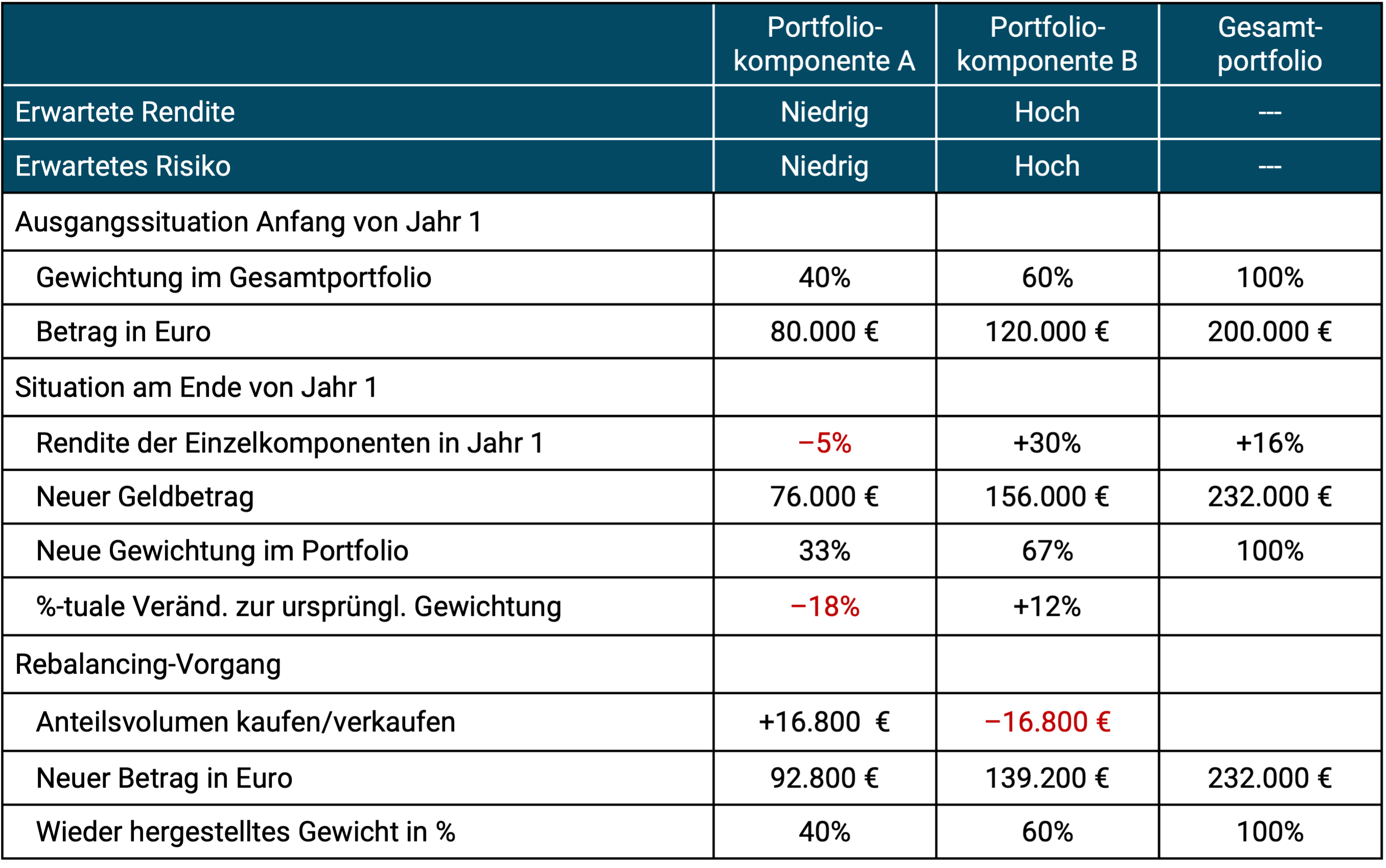
RB has the important function of keeping the return-risk character, i.e. the opportunity-risk profile of the investor's portfolio over time, in the corridor that the investor's household has consciously chosen - i.e. not allowing this return-risk character to change too much due to market developments (which the investor's household does not influence).
We go into this traditional understanding of RB in much more detail than here in our blog post “Rebalancing: Advantages, Methods, Principles” from December 2021 (see here).
The innovation: “Safe Asset Floor Rebalancing”
In addition to this well-known, “traditional” RB method, there is also a completely different, simpler method that is less well known and which we present in this article. We call this alternative approach Safe Asset Floor Rebalancing (SAF-RB). [2] It is to be distinguished from the traditional RB method described above, which we will refer to below as T-RB for the sake of brevity.
The central feature of the T-RB is the percentage shares for the individual port components set by the investor at the beginning of the period. That's why T-RB is also one of the names in English Constant Proportion Rebalancing or Fixed Percentages Rebalancing known. In SAF-RB, however, there are no constant percentage proportions.
The easiest way to describe SAF-RB is to use a mini case study. We are taking on the couple Leonhard and Laura Bergmüller. Beide sind 50 Jahre alt und leben in NRW. The Bergmüllers' combined net income is 6,000 euros per month. They can live comfortably on this and still save 500 euros a month for retirement purposes. The Bergmüllers' three children have left the house and are financially independent. Both spouses are employed and want to work until they are 65 – around 15 more years. Die Bergmüllers leben zur Miete. Their total joint assets are 670,000 euros. It comes from savings over the past 20 years and a gift from Laura's parents. The 670,000 euros are in a bank account and in a bank deposit. Schulden haben die Bergmüllers nicht. The married couple's combined human capital - the financial mathematical present value of the expected joint net salary income until the planned end of working life - is approximately 850,000 euros and is therefore, as with most households that are still working, higher than the financial and real estate assets after deducting debts. [3] It should be emphasized that human capital is a low-risk asset for normal employees.
At this point in their lives, the Bergmüllers have chosen one Safe asset floor (SAF) of 200,000 euros. The SAF corresponds to the volume of “safe assets” that Leonhard and Laura currently consider to be appropriate for them to have sufficient financial peace of mind. Why 200,000 euros? This is the amount of money with which the Bergmüllers could finance their current living expenses for a full three years if their professional income suddenly fell to zero and there was no other replacement income, e.g. B. from unemployment benefit/citizen benefit. The number 200,000 euros results from the average monthly living costs of 5,500 euros × 12 months × 3 years = 198,000 euros. [4] Ultimately, the specific level of this target amount is arbitrary or subjective. Another couple would probably have chosen a higher or lower SAF.
The Bergmüllers invest these 200,000 euros in Safe Assets, in this case in an interest-bearing daily money of 50,000 euros at an online bank in Germany and in a money market fund ETF of 150,000 euros, i.e. an index fund super safe short-term high-quality bonds (government bonds and/or corporate bonds). For more on money market funds see here in our blog post “Money market funds – the smart alternative to overnight money”. The amount of the daily allowance is within the statutory deposit insurance limit of 200,000 euros for the couple and can therefore be classified as very safe.
Mandatory characteristics/requirements for the “safe asset” are: (a) Default risk that can no longer be reduced further (credit risk), [5] (b) no or almost no volatility risk (value fluctuation risk), (c) maximum liquidity (the asset must always be convertible into cash within a few days without significant transaction costs) and (d) no exchange rate risk.
We know from the global capital market history of the last 120 years that such safe assets, after deducting inflation, taxes and costs, provide a long-term return that is close to zero. This low return is the price for their maximum security and maximum liquidity. The fact that this real net return is so low in the long term has little or nothing to do with the interest rate policy of the central banks, although many “experts” have been saying this for years. We describe the economic background here.
The Bergmüllers invest 100% of the remaining 470,000 euros from their total assets of 670,000 euros, as well as the monthly savings rate of 500 euros, in globally diversified stock ETFs. 200,000 euros in safe assets and 470,000 in the risky part of the portfolio gives a percentage asset allocation of (rounded) 70/30.
Let us now assume that the Bergmüllers receive an inheritance of 330,000 euros in cash from Leonhard's recently deceased great aunt in Canada (inheritance taxes already deducted). The couple's total assets grow from 670,000 euros to one million. The question arises as to how these new funds should be invested (larger additional investments always lead to the question of rebalancing).
Comparison: Safe Asset Floor Rebalancing and Traditional RB
In Table 2 below we illustrate the difference between the two rebalancing approaches - again using the case study of the Bergmüller couple. T-RB assumes that the Bergmüllers maintain their original (initial) percentage asset allocation of 70/30 after receiving the inheritance of 330,000 euros. At SAF-RB, on the other hand, the Bergmüllers keep their safe asset floor constant and invest the entire inheritance in the risky part of the portfolio. This results in a significant shift in the percentage portfolio structure.
Table 2: Bergmüller couple: Comparison of traditional rebalancing and SAF rebalancing
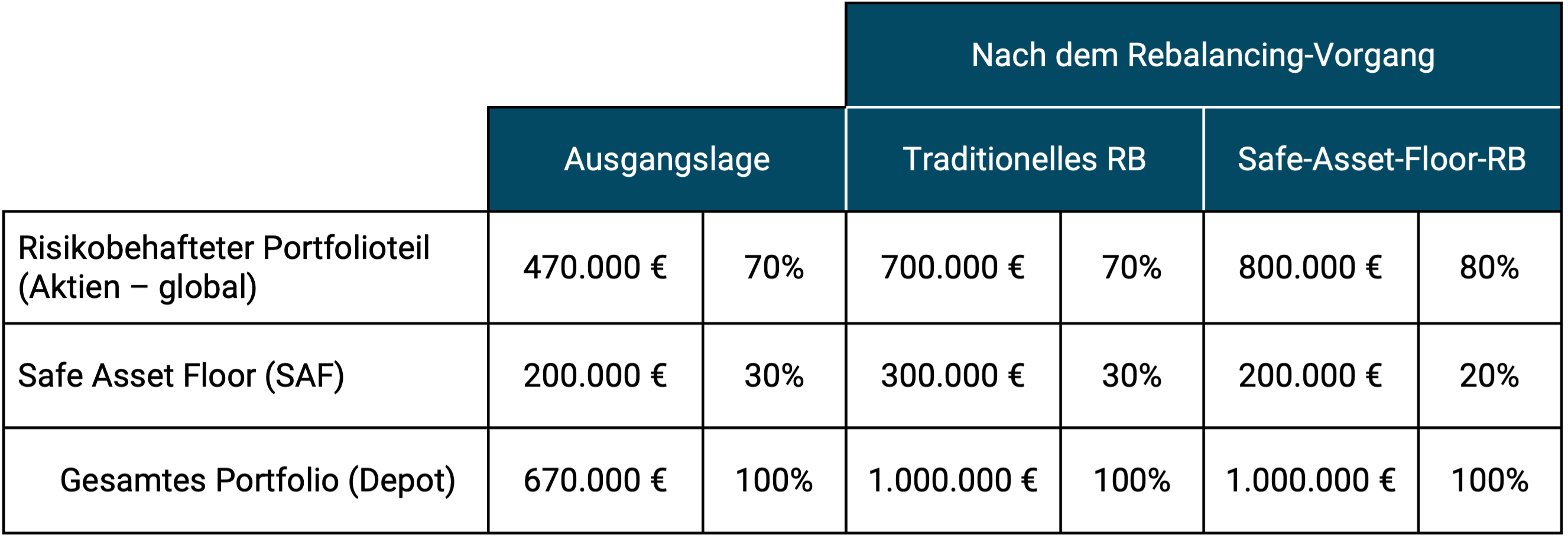
► Without costs and taxes. ► Monetary amounts rounded to the nearest thousand.
The logic behind Safe Asset Floor Rebalancing
What is the economic logic of SAF-RB and how does it differ from the logic behind traditional RB?
Behind SAF-RB is the financial economic concept Asset Liability Matching, also Asset Liability Management called. That sounds complicated, but it isn't. Think of a household like a small business with a balance sheet. On the left side of the balance sheet (which can be visualized as a T-account) are the assets and on the right side are the liabilities, the liabilities or obligations to the investors (debt and equity). For a natural person, these obligations can be thought of as the sum of future living expenses (or more precisely, the present value of this sum discounted to the present). Since these living costs will most certainly actually be incurred at the expected level (e.g. will not decrease due to market influences or other factors), these future “liabilities” should be offset by an asset on the left side of the balance sheet, which will also never fall in value with maximum certainty, i.e. the safe asset. This is the basic idea behind asset liability matching. Its purpose is risk management or risk reduction. [6]
In the case of a household that still receives professional income, i.e. that has not yet entered retirement and in which it has to “tap” at least some of its assets to cover living expenses, the quantification of the SAF in terms of size is ultimately subjective/arbitrary. The specific size of the amount depends on the individual security needs of the household and its financial possibilities - see the example of the Bergmüllers described above.
However, for a household that no longer receives any professional income and whose human capital has fallen to zero (e.g. a pensioner household), it is quite easy to formulate a simple, somewhat objective rule of thumb for “sizing” the SAF target value.
In general, SAF-RB is more explicit than T-RB absolute The magnitude of the portfolio components (sizes measured in monetary units), less on the relative percentage structure like T-RB. This different basic philosophy may correspond to the intuitive perception of risk of many private investors.
Determine your SAF target value
It works like this: Each household member calculates their remaining life expectancy. There are numerous easy-to-use web-based calculators, such as this one here. Four to five years should be added to the calculated “average remaining life expectancy”. Then you are approximately at the value that you will not exceed with an 80% probability (instead of a 50% probability in the case of the average remaining life expectancy).
If you want to be very careful, i.e. very conservative, you take this number - let's say it is 30 years - and multiply it by the total annual living costs, which cannot be financed from other very secure sources (such as the statutory pension insurance).
Another mini case study: Ricarda is single and 60 years old. She recently finished her career. Ricarda's calculated mean remaining life expectancy is 29 years (up to age 89). Ricarda adds five years - as recommended above - to arrive at an age value that she will only exceed with an approximate 20% probability. This results in a calculated remaining lifespan of 34 years. Ricarda's pension gap - the gap between her desired monthly standard of living and her civil servant pension - is 900 euros per month. This means we arrive at a maximum SAF target value of 900 euros × 12 × 34 = 367,000 euros (rounded). [7] Ricarda's liquid assets are 500,000 euros. This means that Ricarda, who we assume wants to be “very safe”, invests 367,000 euros in safe assets (see above) and the rest (133,000 euros) in a globally diversified equity ETF.
If Ricarda were less conservative (less risk-averse) or if her financial options were more limited, she could be content with covering the cost of living gap for 20 years or 15 years through her safe asset floor, since we can assume that in 15 or 20 years at the latest, the stock portion of her portfolio will with a high degree of probability (but by no means with 100% probability) be worth the same or more, adjusted for inflation, than it was at the start. [8]
Let us now also assume that Ricarda has a very good year in stocks with her stock ETF investment in the first year of retirement and earns 25% (33,000 euros). In a SAF-RB concept, she leaves her portfolio unchanged in the following year (we assume that the SAF value remained unchanged after inflation, taxes and costs). In general, in the SAF-RB world it allows the risky portion of the portfolio to grow or shrink as desired over time. In principle, its percentage weight in the overall portfolio can change freely in any direction.
Since the equity asset class has a significantly higher expected return than safe assets (as we have defined them here), the equity weight should increase over time. Reallocations to keep the percentage asset allocation constant, as with traditional RB, do not occur with SAF-RB.
Ricarda takes the annual funds to cover her pension gap (900 euros × 12 = 10,800 euros) from the SAF part of her portfolio, because with each new year her remaining life expectancy decreases by (approximately) one year and the safe asset floor can be reduced accordingly in parallel. At least that is the removal procedure if you stick closely to the SAF philosophy. If desired, Ricarda could also withdraw the 10,800 euros annually from the stock portion of her portfolio, depending on her personal preference. Then the level of security of their portfolio would increase moving forward.
The two case studies should make it clear that a “clear mathematical rule” for determining the SAF target value only exists for households that are no longer working (whose human capital has fallen to zero) and need to make withdrawals from their liquid assets in order to (co-)finance living expenses. For these households, the amount of the SAF is calculated using the formula described above, depending on the remaining life expectancy and the assets to cover living costs. If the latter requirement does not exist (all living costs can easily be covered from other sources such as the statutory pension or rental income), the SAF could be set very low and only include the usual “personal liquidity reserve” (see below).
For employee households that still receive income from work and therefore still have positive, low-risk human capital, the SAF target value is determined, as mentioned above, purely subjectively and depending on the individual case - without any general mathematical rule.
Further implementation aspects of SAF-RB
How should the factor of inflation be assessed in the cost of living and thus in “SAF sizing”? As suggested above, we can expect the SAF component to recoup inflation (but not much more) in the long run, net of costs and taxes, with almost zero volatility.
If, exceptionally, the inflation-adjusted net return of the SAF is significantly negative over several years, the SAF in the portfolio may need to be increased, either by directing savings rates into the safe asset component (if the household is still in the savings/asset accumulation phase) or by reallocating it from the risky part of the portfolio (if no more savings rates are flowing). Such an increase in the SAF in the portfolio may also be necessary if a household increases its standard of living over time. In principle, a household should check the level of the safe asset floor in its portfolio every year and adjust it upwards or downwards if necessary.
The “personal liquidity reserve” (the “nest egg”) recommended in many financial advice books and by all financial advisors for private households of e.g. B. three to twelve times the average monthly cost of living should be considered part of the safe asset floor.
SAF-RB refers exclusively to the highest portfolio level, i.e. the division of a passively managed portfolio into (a) “risk-free” assets (the safe asset floor) and (b) risky portfolio parts, i.e. all ETFs that reflect the global stock market and possibly other risky admixtures such as emerging market bonds, raw materials, gold or crypto. In Gerd Kommer’s world portfolio concept, this corresponds to “Level 1 asset allocation”. At the underlying, deeper structural level, the level of individual ETFs or other forms of investment, traditional RB must still be practiced - in addition - even when SAF-RB is used. The total workload with SAF-RB will still be lower than if only T-RB takes place alone.
Of course, in individual cases, other criteria are conceivable that determine the SAF target value. However, for reasons of space, we will not go into this.
What are the advantages and disadvantages of SAF rebalancing relative to traditional rebalancing?
Advantages and Disadvantages of Safe Asset Floor Rebalancing
The advantages of SAF-RB:
- SAF-RB can be a suitable alternative for those private investors who are reluctant to use traditional RB because they find it too rigid and too theoretical. At the same time, SAF-RB represents a sufficiently formalized set of rules with a simple but convincing economic logic behind it, so that the accusation of rule-free arbitrariness without guard rails that are recognizable to everyone involved and without logic does not hold.
- With SAF-RB, the emotionally difficult situation of “selling winners to buy losers” occurs less frequently than with traditional RB.
- Given an identical starting asset allocation and a sufficiently large portfolio, SAF-RB statistically results in a higher final asset value than traditional RB. The heirs of the asset owner can be happy about this.
- SAF-RB reduces the number of rebalancing-induced trades. This lowers transaction costs (costs of buying and selling) and reduces work. Likewise, at SAF, price gains are realized less frequently in the equity portion of the portfolio. This can result in tax advantages (see here).
- SAF-RB can work particularly well for very wealthy households, as by definition they will never have the problem of being able to fully finance their desired volume for the safe asset floor. In addition, very wealthy households often have a higher tolerance for portfolio volatility than less wealthy households.
- However, SAF-RB can also represent a useful solution for novice investors with no experience in the capital market (both those with a small or large portfolio) if they are not yet familiar with the stock market or other risky asset classes or with their own mental risk-bearing capacity. The safe asset floor could initially be set relatively high in relation to the total assets in order to give yourself sufficient peace of mind and at the same time start (so to speak approach) with risky investments (such as stocks) on a smaller scale, instead of continuing to remain on the “edge of the playing field”. In the standard case, the share of the risky portfolio component would gradually increase as a result of a long-term positive price development of the risky assets and through subsequent investments in them (e.g. through an ETF savings plan), as a result of which the investor household gradually grows into an increasingly opportunity-oriented portfolio.
The disadvantages of SAF-RB:
- Under typical circumstances, SAF-RB leads to higher portfolio volatility and higher drawdowns in monetary terms in the long term because the percentage of risky portfolio components in the overall portfolio increases over time. To put this into perspective, one must add that the increased volatility (the “volatility delta” to a T-RB portfolio) in absolute monetary units (rather than percentage values) will probably be within previously accumulated profits.
- For young households that are still at the very beginning of the portfolio building process and generally for households that are still working (i.e. still have positive human capital), the SAF philosophy provides less clear indications (in the sense of quantifiable, generalizable criteria) as to how high the safe asset floor should be. For these households, the sizing of the SAF usually has to be carried out according to purely subjective, case-specific criteria.
In addition to these disadvantages, a critic of SAF-RB could also object that this is not a real rebalancing at all, since there is no periodic return to a fixed portfolio structure after it changes from its position due to market effects ex ante the chosen proportions. From a formal point of view, this objection is correct, but substantively it is wrong, because SAF-RB does represent a rules-based control plan for the development of the portfolio structure over time. However, this plan is based on fundamentally different principles than those of T-RB. There are no fixed percentage values for the top portfolio structure at SAF-RB, only a safe asset floor that is fixed in absolute numbers.
It should be noted that for portfolios that do not experience any significant additions (re-investments) or withdrawals, the difference between SAF-RB and T-RB will generally be small in the short and medium term.
Conclusion
We view Safe Asset Floor Rebalancing as a viable alternative to traditional rebalancing for ordinary retail investor households. SAF-RB fits well with the risk management intuition of many retail investors. In the long term, it typically leads to a higher final portfolio value because the low-yielding safe assets have a smaller portfolio share on average over the entire period. SAF-RB tends to require fewer “trades”, which can be a cost and tax advantage, especially in a portfolio in which there are no ongoing additions (additional investments) or ongoing disinvestments (withdrawals). A disadvantage of SAF-RB is that it leads to more volatility and higher drawdowns measured in monetary units in the long term.
Endnotes
[1] From an economic perspective, distributions (dividends, interest) that are not immediately reinvested also correspond to withdrawals.
[2] Safe Asset Floor = “floor of safe assets”.
[3] On the information portal www.finanzfluss.de There is a free human capital calculator.
[4] Cost of living here really means all living expenses, including average amounts for “lumpy expenses” that only occur every few years, such as: B. for the purchase of a new car or larger maintenance costs for an owner-occupied residential property.
[5] Bank balances above the state/statutory deposit insurance limit of 100,000 euros per bank-customer combination do not meet this criterion.
[6] In the English-language specialist literature on institutional investing (in contrast to private household investment), concepts that have similarities to the SAF-RB approach outlined here are sometimes referred to as Liability Matching Portfolios (LMP) or Liability Driven Investing (LDI). Otherwise, we are not aware of any specialist literature specific to the SAF-RB approach for private household investment. The terms “Safe Asset Floor” and “Safe Asset Floor Rebalancing” come from us.
[7] The author William Bernstein mentions these costs in his guide books Residual Living Expenses. When it comes to quantifying them, he suggests the same approach as we do here.
[8] The prerequisite for this assumption is a systematically globally diversified stock portfolio. For individual values (including, for example, 30 different individual values), the return risk would be much higher.