Save taxes through buy-and-hold

From Gerd Kommer and  Jonas Schweizer

This post was updated in November 2024.

The vast majority of our readers now know that buy-and-hold (“B&H”) helps to keep the additional costs of a capital market portfolio low. Low additional costs, in turn, all other things being equal, lead to significantly higher final assets in the long term. 

However, far too few private investors know this Tax advantage from B&H, which – as well as low ongoing costs – results in a significant improvement in net returns and final assets.

Are you already convinced of buy-and-hold, but don't have the time or desire to implement it? We have Gerd Kommer's 1 ETF solution: The L&G Gerd Kommer Multifactor Equity UCITS ETF. Find out more >

Most of us are aware that it is economically advantageous to postpone a given tax payment into the future, if legally permissible. This is often justified by the need to prevent the outflow of “tax liquidity”. However, this explanation, which has even been put forward by tax advisors, is at best half correct. Only half-true, because it exaggerates a mostly rather unimportant peripheral aspect - the postponement of an outflow of liquidity that will take place at some point anyway - into the main explanation. The actual main explanation for the economic advantage of deferring tax payments into the future is the tax effect it creates Present value effect. We'll explain what's behind it below.

As is well known, price gains on shares are only taxed when they are realized, i.e. at the time of sale. In technical jargon this is called the “subsequent taxation of capital gains”. It is to be distinguished from the ongoing, “immediate” taxation of dividends. Dividends are always taxed immediately or annually. This applies to dividends for individual stocks as well as for stock funds. (In the case of investment funds, including ETFs, the distinction between distributing or accumulating funds is in principle irrelevant, although - keyword "advance flat rate method" for accumulating funds - there are small differences in the effective level of taxation.)

The easiest way to understand B&H's tax present value effect is to explain it with hard numbers. We assume that a share The dividend yield of 2.5% assumed here corresponds almost exactly to the average value for the MSCI World index over the past 25 years.

As we'll see in a moment, it makes for the effective Tax rate and thus the actual after-tax return makes an enormous difference whether the 7% price return is taxed at the end of each calendar year - like with a typical active investor - or only after, for example, 30 years when the share or ETF share is sold - like with a disciplined B&H investor.

For a typical active investor, the capital gains are taxed annually (“immediately”) because he holds most of his securities for less than twelve months or at least not much more than twelve months, i.e. he realizes profits more or less continuously.

In contrast, for a disciplined B&H investor, taxation, the actual transfer of the “deferred tax liability” incurred with every euro of capital gain, occurs perhaps only after 20 or 30 years or even later, when the investment is sold because the investor or his heirs want to consume the proceeds or use them for other purposes. 

Now the financial crux: Due to the subsequent taxation of price gains in the case of B&H, which is not annual, the investor can only pay the tax amount that he or she has to pay in a given year not has to pay, continues to invest afterwards, so that this amount continues to work for him and thus produces income. This would not have happened with immediate annual taxation, although here too the (same) tax amount has to be transferred to the state at the very end of the observation period. This often overlooked detail creates the cash value tax benefit. (A general explanation of the economic present value method can be found at the end of this blog post for readers who are new to it and want to understand the issue in detail.)

A calculation example: We assume that Lena and Carla have a stock portfolio worth 10,000 euros. Both achieve a 10% price return in year 1 and another 10% price return in year 2 (we are not interested in the dividend yield here). Lena is a speculatively oriented “active” investor who usually only holds a security for a few months, while Carla is a consistent buy-and-hold advocate whose “favorite holding period” corresponds to Warren Buffet’s: “forever.” 

As mentioned, Lena and Carla both achieved price gains of 10% in year 1, i.e. 1,000 euros. Lena, the “trader”, pays 26.4% (264 euros) of this to the state in the first year as capital gains tax + contributions (all amounts rounded to full euros). She has 736 euros left of her pre-tax profit, which she can use to move into the second year of investment.

Carla doesn't pay any taxes because she hasn't realized any profits. Carla goes into year 2 with the full (untaxed) profit of 1,000 euros.

In year 2, Lena only earns 10% × 736 euros = 74 euros with her already taxed profit from year 1, while Carla earns 10% × 1,000 euros = 100 euros. In the second year, Carla earned 26 euros (the difference between 100 euros and 74 euros), which Lena finally earned not has and never will have. In addition, the above-mentioned 264 euros (1,000 euros minus 736 euros) remain in Carla's portfolio and can continue to produce good returns in the third and subsequent years. 

If we repeat this game for 30 years and also take into account the compound interest effect (which was omitted in the above description of year 1 and year 2 for the sake of simplicity), then the initially modest difference between Lena and Carla ultimately results in an astonishing final wealth advantage for Carla.

Warren Buffett calls the downstream taxation of price gains in buy-and-hold an “interest-free loan from the government” and economically it is exactly that. The B&H investor receives new interest-free loans from the government almost every year, each in the amount of the deferred payment of his tax debts incurred in previous years, which has been postponed into the future. He will only have to repay these loans when the assets are sold many years from now, but in the meantime he can invest these loans and let them work for him.

The following table quantifies the tax present value advantage for shares under German capital gains tax for different periods of up to 40 years. As described at the beginning, a total return of 9.5% p.a. is assumed, which is divided into a 7% price return and a 2.5% dividend yield. The “statutory” (legal) tax rate is 26.375% (rounded 26.4%) and results from 25% capital gains tax + 5.5% solidarity surcharge on this 25%. The statutory tax rate is offset by the effective tax rate, and this decreases for B&H investors with each additional buy-and-hold year. For active investors, the statutory and effective tax rates are identical.

Table: The tax present value advantage for stock investments through buy-and-hold – Assuming an initial one-off investment of 100 euros (all numbers rounded)

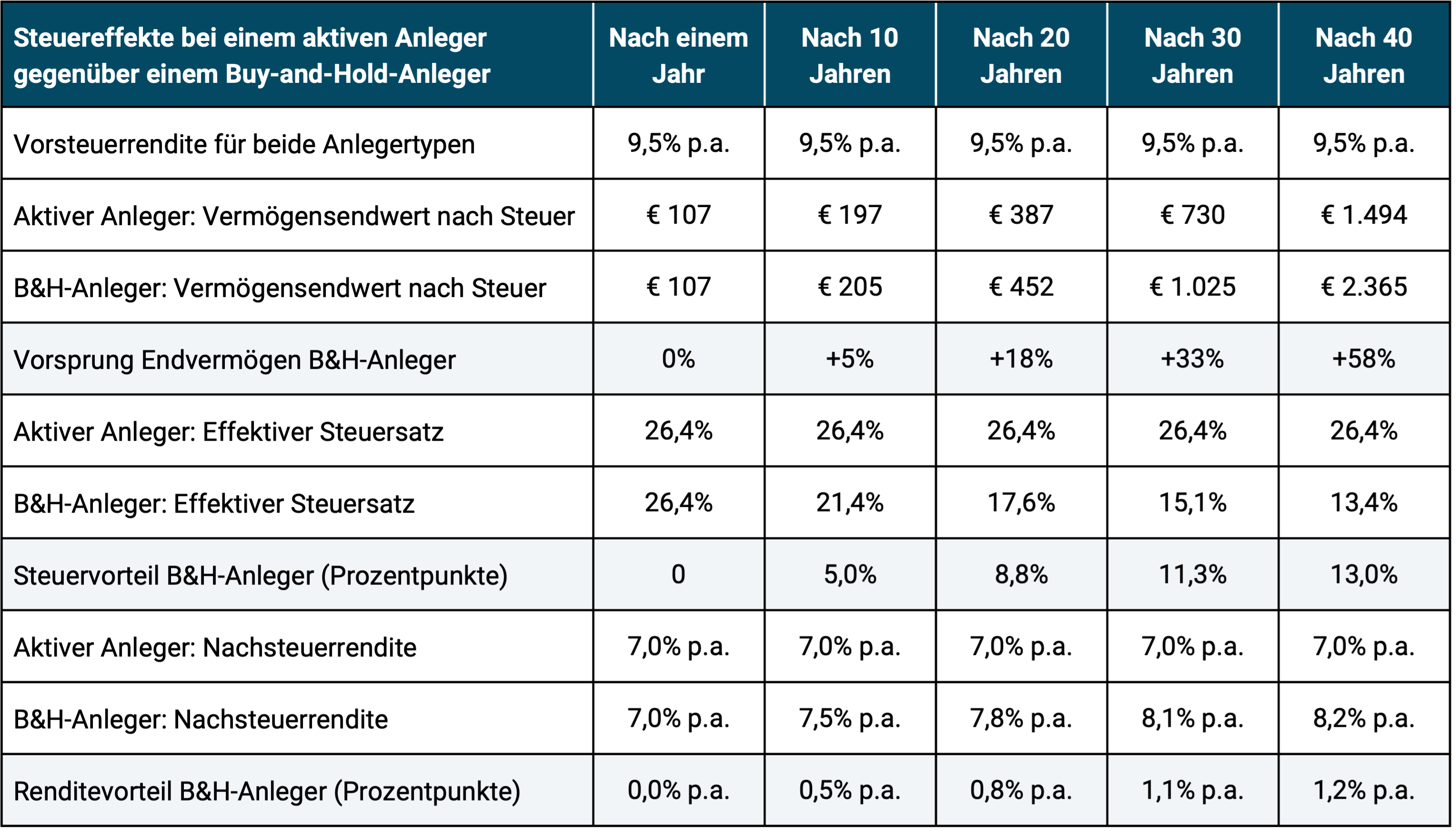
The calculation example in the table illustrates that under the current withholding tax, a B&H investor receives an average net return over a 30-year period that is 1.1 percentage points annually (8.1% p.a. instead of 7.0% p.a.) higher than the net return of an investor who does not have this tax present value advantage because he buys and sells his securities more or less annually. This has a huge impact on the final value of assets due to the compound interest effect. For the B&H investor it is 33% higher after 30 years and 58% higher after 40 years.

The table does not even take into account the savings through B&H, which result from the lower transaction costs for buying and selling, as we are only concerned with tax effects here.

What else is there to know about the tax present value effect of buy-and-hold?

This tax advantage is greater the higher the underlying tax rate is. If the German withholding tax were to be replaced - as some parties represented in the Bundestag are advocating - by the normal (progressive) income tax rate, which is higher for most investors, the relative benefit of B&H for most investors would increase even further. A numerical example: With an observation period of 30 years and a tax rate of 35% (instead of 26.4%), the B&H investor's final wealth advantage increases from the previous 28% to 36% and the annual net return advantage increases from 0.8 percentage points to 1.1 percentage points.

B&H's tax benefit also increases with the level of the underlying nominal appreciation yield. For example, if inflation were to increase significantly over the long term and therefore nominal stock returns were to rise in parallel over the longer term (this is the usual economic context), the B&H tax advantage would also be greater.

The periodic rebalancing, which also makes sense for a B&H investor and which we advocate, slightly reduces the extent of the tax present value advantage. [1] This effect was not taken into account in our calculation. Fortunately, this restriction does not apply to so-called cash flow-based rebalancing - the use of cash flows that are already taking place into the portfolio (asset creation phase) or out of the portfolio (asset use phase) for rebalancing purposes.

Saving taxes with B&H is easy and works 100% reliably. It's not a tax loophole and you don't need a tax advisor. This tax advantage exists in every country in which capital gains are taxed. It is therefore not specifically related to the German withholding tax (capital gains tax). This tax advantage is not threatened by the currently known taxation plans of the parties in the Bundestag, which are aiming for tax increases, but could even become greater.

Conclusion

Buy-and-hold has three major return benefits, but only one of them - saving on transaction costs (buy/sell) - is truly widely known. However, only a few private investors are aware of the economically important advantage from the tax cash value effect. (We will discuss the third major advantage of B&H, the avoidance of harmful timing effects from “performance chasing,” in a separate article in the next few months.)

Why do we hear so little about B&H's tax advantage from the financial industry and the financial media?

Banks and non-bank asset managers usually remain silent on this topic because the use of this tax saving strategy by their customers is detrimental to their profits. The financial sector earns much more from the actionistic back and forth, from getting in and out of potatoes. Furthermore, their fables about active investing as a way to achieve high returns or as a tool for risk protection do not fit with B&H. We know that these are just fables from financial market research, which has proven the statistical under-return of active investing in studies that can no longer be counted.

For most financial journalists and finfluencers, the topic of tax cash value benefits is too complicated, too unsexy and therefore not worth reporting on.

Endnotes

[1] Rebalancing is the purely mechanical return of a passive portfolio to its original asset allocation, its percentage division into asset classes. This reduction is necessary if there have been shifts in its structure over time because the individual components of the portfolio had different returns.