
<<< This blog post is also available as a YouTube video. >>>
From Alexander Weis and Gerd Kommer
This post was slightly modified in January 2025 and was until then titled “Timing the market entry – does it work?”
Anyone who wants to invest a significant amount in the stock market almost inevitably asks themselves the question: “Is now the right time to buy stocks?” Our gut feeling almost always says no, because if prices have risen significantly in the past, we fear that we are investing in an overpriced market or – even worse – that we are entering shortly before a crash. If the prices have fallen in the last few months, we believe that we are “grasping into a falling knife”, as the hackneyed stock market saying goes, i.e. investing in a market that is falling even further. Felt our entry always comes too early.
In this post we look at “type one” fear: the fear of entering a market that is too expensive or a market that is about to experience a sharp downturn. [1]
A solution that we hear again and again for this ultimately old question is to simply wait until the stock market - measured against a broad index - has collapsed by a certain percentage (e.g. 20% or 30%) before investing and only then invest in the now significantly cheaper market. This investment strategy is often referred to in English as “buy the dip”. [2]
Buy when the cannons are roaring
According to this consideration, the investor defines a percentage “loss threshold” relative to the index level at the starting point, which must be reached (“torn”) before he can withdraw his money from a safe investment – e.g. B. the asset class “cash” is reallocated into shares. Cash means a low-interest money market investment, e.g. B. a call money or a money market fund. This “investment reserve” is often referred to as “dry powder” in the context of the “buy-the-dip” approach – a term that refers to the “gunpowder” held on hand that remains dry and therefore ready for use.
If the percentage loss threshold is reached due to the market collapse, the investor enters the market more cheaply after reaching the loss threshold than he would have done with the alternative “invest immediately without waiting combined with subsequent buy-and-hold”.
We call this market timing approach “mechanical loss threshold timing” (MVT).
The investor determines the level of the loss threshold relative to the stock index level at the beginning of the observation period as desired. The loss threshold is a specific index level below the level at the start of the investment period. (For explanation: With a loss threshold of 30% and an index level of 100 euros at the beginning of the evaluation period, you would then enter the market as soon as the price fell to 70 euros.)
This simple, rules-based, countercyclical strategy does not require time- and labor-intensive “valuation exercises” (such as continually reassessing the market P/E [price-to-earnings ratio]). The simplicity of the strategy also lies in the fact that it is related to investing Dry powder In stocks there is only a single waiting phase at the beginning. Naturally, their duration is not known ex ante. Once the loss threshold has been reached and the “entry” has been completed, the investor remains fully invested in stocks for the remainder of the observation period and from this point on no longer differs from the “immediate all-in benchmark” (hereinafter abbreviated as “SAI”).
As mentioned at the beginning, MVT is a variant of the well-known “buy-the-dip” approach. A variant in that a classic buy-the-dip strategy – strictly speaking – also requires a criterion for a partial sale, i.e. a partial exit, for the phase after the market recovery (restoration of the dry powder). For reasons of simplicity and brevity, we will omit it in this blog post.
Two possible outcomes: loss threshold is broken or is not broken
To put it simply, the MVT strategy produces only two ideal results: (a) the loss threshold breaks after not too long; then the MVT strategy will beat the SAI strategy with mathematical necessity over the entire period; at least in a world without rebalancing (see below). (b) The loss threshold does not break; then the MVT strategy will be subject to the SAI strategy over the entire period. If the loss threshold does not break in the first few years after the start, this breaking becomes increasingly unlikely for each subsequent year, as an increasingly larger “buffer” tends to build up with each passing month.
The MVT idea seems clever at first glance. We try to evaluate whether it really is using a “back test” (testing based on historical data). We use the historical monthly returns of the global stock market from 1970 to 2018 (49 years), which has an average nominal return of 7.5% p.a. during this period. a. produced (real 4.7% p.a.). (1970 is the start date for data availability reasons.)
In our backtest, we determine for each individual starting month within the period 1970 to 2018 (49 years or 588 months) whether a predefined percentage loss threshold after the starting month would have ever been broken in the remaining period up to December 31, 2018. The first scenario starts on January 1, 1970 (it's 49 years long), the last one starts on December 1, 2018 (it's only a month away). Considering that we are testing ten different loss thresholds from 5% to 50% (at 5% intervals), this gives a total of 10 × 588 = 5,880 individual historical scenarios.
It should be mentioned in this context that percentage loss thresholds for such an MVT strategy only make sense in practice in nominal, not inflation-adjusted (real) values. A definition in real numbers would ultimately lead to unnecessary implementation problems and would only change the overall results slightly (we also tested this). For reasons of space, we will not go into this aspect further.
What exactly did we do? For each of the 588 calendar months for loss thresholds ranging from 5% to 50%, we answered the question: “Will the historical loss threshold ever break or not from this starting month through December 2018?” A loss threshold of e.g. B. 10% is considered to have been broken if the index level measured at the start of the MVT strategy is subsequently undercut by 10% or more in a single month. For a loss threshold of 10%, this was the case in 296 of the 588 months (49 years), which corresponds to an “MVT success rate” of around 50%. We repeated the same calculation for the other loss thresholds from 5% to 50% and summarized the results in the following graphic. The horizontal axis (x-axis) indicates the chosen loss threshold; the vertical axis (y-axis) on the left (and associated bars in blue) describes the number of cases in which the MVT strategy would have worked (“probability of success”); The y-axis on the right (and the corresponding bars in red) shows the average annual additional return that could have been earned each year if the MVT strategy was successful - and only then.
Figure: Historical probability of success (left vertical axis) and annual excess return (right vertical axis) of the MVT strategy for different loss thresholds (horizontal axis) compared to the simple SAI strategy based on historical monthly returns from 1970 to 2018 (49 years)
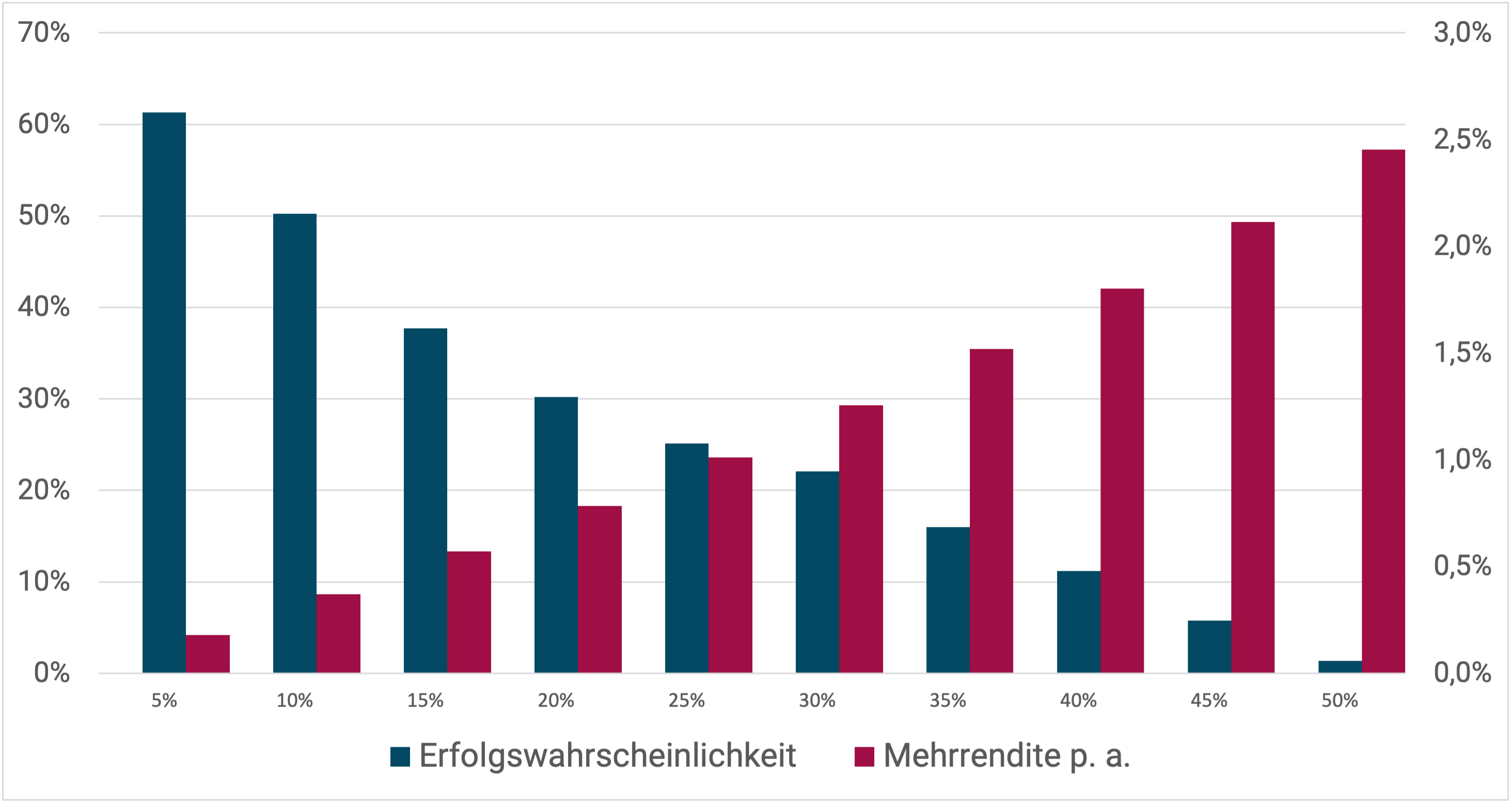
Source: Own calculations using data from MSCI. ► “MVT” stands for “mechanical loss threshold timing”; “SAI” for “Immediate All-In” i.e. “Invest immediately without waiting (combined with buy-and-hold)”. ► Data: Global stock market from 1970 to 2018 in DM/EUR. Since the broadest global stock index available, the MSCI ACWI IMI, is only available from 1996, we used the MSCI ACWI standard for the period 1988 to 1995 and the MSCI World Standard for the period 1970 to 1987. ► Without taking transaction costs and taxes into account. ► Historical returns provide no guarantee of a similar repeat in the future.
Take a moment to examine the graphic in more detail. Even with low loss thresholds, the MVT strategy fails surprisingly often. Let's look at the loss threshold of 5% as an example: Here MVT failed in 38% of all cases (= 100% - 62%). At high loss thresholds, the proportion of failures is even greater; For example, with a loss threshold of 35%, MVT fails in 84% of all scenarios. Failure scenarios lead to high lost profits (“opportunity costs”). These lost profits consist of the difference between the stock market return and the cash (money market) return over the entire duration of the scenario - which could be several decades, depending on the scenario.
The lower (milder) the loss threshold is set, the sooner it will be reached (broken), but the additional return that can be achieved with it will be more modest.
There is no need to consider loss thresholds of 55% and more, at least in this test, because in the last 49 years there has never been a cumulative loss (“maximum drawdown”) of more than 53% nominally in a global stock index.
Overall assessment of the MVT strategy
How should the MVT strategy be assessed overall? This question can be answered by comparing the expected excess return if the MVT strategy works with the expected underreturn if it fails. With the simple SAI strategy you would have an average nominal return of 7.5% p.a. over the last 49 years. a. achieved. Using the MVT strategy and a loss threshold of 30%, in the event of success (but only then), an average return of 8.8% (7.5% + 1.3%) would have been achieved. If the loss threshold is not exceeded, the return achieved corresponds to the money market return for the respective period, since the money was never invested and, as assumed, “always remained in the bank account”. We assume a nominal return of 3% p.a. for this return. a. Since the probability of success is only 20% with a loss threshold of 30%, we get a probability-weighted MVT return of around 4.2% p.a. a. (≈ 20% × 8.8% + 80% × 3.0%) - the return of the MVT strategy is therefore expected to be 3.3 percentage points p. a. below that of a SAI investor. After 30 years there is an excess return of 3.3% p.a. a. to a 165% higher final wealth for the SAI investor compared to the MVT investor.
A second calculation example: With a loss threshold of 20% (probability of success 30%), the probability-weighted MVT return is 4.6% p.a. a. (≈ 30% × 8.3% + 70% × 3.0%).
The probability-weighted return
The crux of the matter: MVT's probability-weighted return is below the SAI return for all loss thresholds. Apart from this argument, two other considerations speak against the use of an MVT strategy.
Firstly, with SAI it is possible to continually return a portfolio to its target allocation by means of rebalancing. In times of sharply rising markets, this means nothing other than “bringing price gains to safety”. With disciplined rebalancing, it can happen that an SAI strategy even performs better than a functioning MVT strategy if the price gains are high enough in the corresponding period.
Secondly, from our perspective, MVT is far more difficult to maintain psychologically and emotionally than SAI. Strategies that are abandoned halfway through often produce particularly poor results. In the case of an aborted MVT strategy, this could mean that you have to enter at higher prices than was initially possible. In comparison, SAI is mentally simpler and therefore more likely to be successful from this perspective.
Conclusion
What can be concluded from these findings? In our view, “crash timing” or “buy the dip” is a market timing strategy that sounds good in theory, but works poorly in practice. Hundreds of academic studies have shown this over the past 50 years and our MVT backtest also shows this. A few lucky people will outperform the relevant market with loss threshold timing, but the majority will go further because these investors never invest in the market at all or only at less favorable prices. Market timers are either very fearful or consider themselves particularly competent. In both cases, they waste too much time on the sidelines in the long term. As we all know, you can't win a game from there. Not to mention the greater nervous strain of the “in-out world” and the higher workload.
Of course, many of the key considerations in the simulation here do not apply to those who believe they can reliably predict sharp market downturns and subsequent recoveries in terms of magnitude and timing. While there is little empirical evidence that real, rather than accidental, skill of this kind exists, the majority of private investors will not give up hope. These investors will predominantly earn less money than would be possible through “immediate all-in investing”.
We have another, differently constructed analysis of a similar buy-the-dip approach here carried out.