In this blog post we look at a specific old wives' tale about the financial attractiveness of owner-occupied residential properties, which has been re-proclaimed "twice a year" by most media in Germany and by the real estate industry for decades with headlines such as the following:

• „Property owners have significantly more money in old age than tenants“ – Headline of an article in the news magazine Spiegel from January 13th, 2025
• „Pensioners who own their own home are particularly wealthy“ – Headline of an article on the news portal t-online.de from December 17th, 2025
• „Homeowners accumulate more wealth than renters“ –Press release from the Association of Private Building Societies in 2025.

However, the statement “own-occupied home leads to higher wealth in old age than renting” is not far from the truth. The statement is a picture-perfect case of “lying with statistics.” [1]

Lying by concealing essential information

As we know, you can lie in many ways. One of them is that person A (the liar) formulates a statement B correctly, but deliberately omits essential information in order to cause a false understanding or error on the part of addressee C. So A lures C into a comprehension trap by omitting crucial information from statement B. That is the lie. Children can already master this method. In English it has a nice compact name Context Dropping used.

Context dropping – lying by deliberately omitting, i.e. suppressing crucial additional information – happens when the statement “Pensioner with his own home [2] are statistically wealthier than pensioners who rent.”

Below we show how this deception actually works. The claim that home ownership is among older households causal for a higher net worth (as conveyed in the exemplary publications cited at the beginning through manipulative context dropping), we will henceforth call “the real estate lie”. [3]

At first glance - without the correct context - the real estate lie in question appears to be true: homeowners actually have a statistically higher net worth in old age than renter households. This is shown by the relevant data and no one doubts its formal correctness.

But the crux of the matter: the statistical wealth advantage of homeowner households (EHBs) over renter households has nothing to do with owning their own home. It is entirely due to other causes. So here correlation is confused or swapped with causation. Yes, EHB households are generally wealthier as they get older than renter households, but they Caused This asset advantage is not the home.

Here is an illustration of the manipulative swapping of cause and effect Real estate lie: The wealth of the average Ferrari-owning household in Germany (around 14,500 households) naturally exceeds that of the average non-Ferrari-owning household (around 41 million). Now the question: Was the Ferrari the cause of this wealth advantage? Of course not. The Ferrari has statistically reduced this wealth advantage - without it, the wealth advantage of the Ferrari households would be even greater. Either way, Ferrari ownership was the result of the income and wealth advantage, not its cause. It's the same with home ownership. It is the consequence, not the cause, of a number of actual causal factors.

The real causes of homeowners' wealth advantage

The “real estate propagandists” are betting that their recipients will fall for the manipulated statement and misunderstand correlation as causality.

However, as scientific research shows quite clearly, the actual causes of the wealth advantage of EHB households are as follows: [4]

1) EHB households have a higher lifetime income, i.e. h. the sum of their net income over the entire period of earning capacity is statistically higher than for renter households. The proportion of households with two incomes is higher among EHB households than among renter households.

2) EHB households have a higher percentage propensity to save. A higher percentage of their net income, which is already higher in absolute terms (see number 1), goes into wealth creation than is the case with renter households. This higher propensity to save is also expressed in the willingness to submit to a “positive compulsory savings contract” that is linked to the loan-financed purchase of a home. More on that below.

3) EHBs are more risk-averse in their investment behavior and therefore achieve statistically higher long-term returns in their wealth creation away from their own home. This increased willingness to take risks is also reflected in the higher entrepreneurial rate among EHB households than among renter households (starting a business and entrepreneurship are very risky). The higher risk affinity is probably due, among other things, to the proven higher average financial literacy of EHB households.

4) EHBs receive more frequent, larger and earlier wealth transfers from their parents and grandparents through gifts and inheritances. This often happens by “subsidizing” the equity share when the EHB household first purchases property when it is young.

5) EHB households have lower divorce rates than renter households. Divorces often cause serious financial losses for those involved. We show why and how these asset losses happen here.

6) If a home investment fails individually - for example due to a combination of unemployment and excessive debt - the affected households often lose their home through seizure or forced sale and become renter households again. Paradoxically, particularly poor home investments contribute to the “home ownership lie” analyzed here.

Note that in the list and description of the six main causes of the higher wealth of EHB households, we did not say anything about Why These households have higher incomes, higher savings rates, greater willingness to take risks, higher financial literacy or lower divorce rates. Quite obviously, a large part of these wealth-promoting factors lies in the socialization of the people concerned; a small part could also be genetically determined.

Would you compare tenant groups with EHB groups where the six causes listed above no If there were a difference, it would be shown that renters statistically achieve higher or similar levels of wealth in retirement. [5]

Why higher wealth? Quite simply because renting in conjunction with other forms of wealth creation - above all with a simple, broadly diversified stock portfolio on a buy-and-hold basis - leads to a higher net final wealth than an owner-occupied property in the majority of time frames if the financial-mathematically correct comparison is made. Furthermore: The relative final asset advantage of the “rent + capital market investment” constellation will tend to be greater, the higher the loan share (“leverage”) is in the comparison EHB. We at GKI have shown this for Germany and others for other countries - see here and here.

We probably don't need to explain in detail at this point why the real estate lie has been spread again and again by real estate agents, property developers, real estate influencers and banks for decades. These parties earn directly or indirectly from real estate purchases or their financing.

The “compulsory savings contract” for real estate

In connection with the correlation phenomenon of the higher net wealth of EHB households in old age relative to renters, it is often even said that not People with conflicts of interest, i.e. “people without a real estate agenda”, argue that the higher net assets of EHB households are based to a large extent on the phenomenon of the “positive compulsory savings contract”. This means that an EHB household that, for example, has taken out a loan for 80% of the acquisition costs is obliged to pay the corresponding expenses (loan installments, property tax, insurance, maintenance) month after month until it has been completely repaid - typically after 25 years or more. Otherwise there is a risk that the property will be seized by the bank. Above all, the repayment element in debt service contributes directly to wealth creation: with every euro of repayment, the percentage of equity in the property increases.

A tenant household is not under a comparable pressure to save, according to the theory of the positive compulsory savings contract. As a result, tenant households will often save less overall or temporarily interrupt their savings over a 25-year period for consumption purposes.

Here too, the confusion/swapping of correlation and causality probably plays a role. People with a naturally high tendency to save are represented more frequently among EHB households than among renter households. This is probably because their pre-existing strong willingness/inclination to save makes it easier for them to accept the long-term reduction in consumption that comes with the “compulsory home savings contract”. These EHB households would not have been able to purchase their own home for certain reasons [6] or if they had viewed a home as a comparatively unattractive investment, the majority of them would have been just as disciplined and saved for the long term in other asset classes. So if you look behind the façade of formalities, you can't even speak of "compulsion" for most people or households who submit to the supposed "compulsory" savings contract, because they would save even without real estate.

What does the development of the “homeownership ratio” tell us?

If you realize that in almost all countries in the world and especially in Germany, wealth creation through owner-occupied residential real estate is financially supported by the state more strongly through taxation and transfer payments (cash benefits) than any other form of private wealth creation, and if you assume for a moment - incorrectly - that owner-occupied real estate systematically produces high returns on equity, then the homeownership ratio (HOR) in most countries would have to continue to rise over time. [7]

But that is not the case. In the USA, the HOR is now at 65%, the same level as 30 years ago, although every American president during this time announced during the election campaign that his administration would increase the HOR. The HOR average of the 38 OECD countries has essentially moved sideways over the last 20 years. [8] There has also been stagnation in Germany over the last decade (current level 47%). Before that, the HOR had risen moderately - probably due to the special and one-off effect of reunification in conjunction with significantly falling interest rates at the time - since in the eastern federal states the HOR was only 24% before reunification (today around 33%).

Wealthy Switzerland is probably the only economically developed country in which, compared to other forms of private wealth creation, home ownership has not yet been systematically favored or subsidized by the state - neither through taxes nor in any other way. [9] The HOR there is only around 40% - probably the lowest value globally. This is a strong indicator that the “natural” HOR in a rich country with a functioning, deep, liquid rental market and a high level of tenant protection (as is common in Western Europe) is in the 40% to 60% range, but certainly not 80% or higher - where politicians and the real estate industry would like the HOR to be.

In this context, many politicians and of course the entire real estate industry have been claiming for decades that a high HOR is a sign of national prosperity. This is also the view of most citizens. Nevertheless, this idea is probably wrong. Empirically, poor countries have higher HORs than rich countries, with rare exceptions. Romania and Bulgaria are among the poorest states in the EU, but have HORs of 86% and 95%, well above the level of the other, richer European states. In general, poor developing countries worldwide are more likely to have higher HORs than rich industrialized countries. One of the richest countries in the world, Switzerland, has – as mentioned – the lowest HOR globally. [10]

Trying to increase the HOR through state measures “with all financial force” is therefore likely to be – as in most countries over the last 25 years – a waste of taxpayers’ money, which is also economically detrimental to tenant households, and is therefore socially regressive and tends to increase wealth inequality.

The future development of residential property prices in Germany

How will residential property prices develop in the future?

In order to answer this question, one should first look at their development in the long-term past. In the 55 years from 1970 to the end of 2024, residential property prices in Germany rose by a paltry 0.1% p.a., adjusted for inflation. Yes, in the eleven and a half years from mid-2010 to the beginning of 2022, prices had risen sharply, but in the approximately 40 years before that and in the three and a half years since March/April 2022, the increases in value, adjusted for inflation, looked poor - even in the largest cities of Berlin, Hamburg, Munich and Cologne. Since spring 2022, residential property prices in Germany, adjusted for inflation, have fallen from their peak at the time by 26% (Greix index) by September 2025 and by 17% (Europe index) by December 2025 - the most recent figures available. [11] (We show the long-term historical price development in Germany and twelve other western countries since 1970 here.)

We already know with great certainty that the population in Germany will begin to shrink from around 2030. Slowly at the beginning, then faster and faster. This means that a demographic headwind that will continue to affect the development of residential property prices for decades will continue. This demographic “price suppression effect” is further intensified by the fact that those who leave the real estate market due to death occupy particularly large areas per person at this time due to their age and wealth. So we will not only have a decline in population and a resulting dampening effect on demand, but - in addition to the net new construction - an indirect increase in the supply of space, since the owners and tenants who leave the real estate market occupy far larger areas per person than the young people who enter the real estate market after moving out of their parents' house. This increases the supply of space relative to demand.

It is possible that real estate prices in Germany, which have fallen since 2022, are already the front end of this demographic supply and demand effect. Asset markets generally already price in the developments expected for the future in the present.

Another long-term effect on increasing the supply of living space, although its strength is difficult to estimate, could result from the conversion of vacant office space into residential space. (It is also conceivable that in the next few years an AI-related loss of administrative jobs will lead to a second wave of reductions in the need for office space after Corona.)

Government actions to combat climate change will also tend to have a detrimental impact on housing prices and returns in the future. At least that's what Allianz writes in Allianz Global Wealth Report 2024. [12] We consider this assessment to be plausible.

Conclusion

There are many over-optimistic myths circulating about the financial attractiveness of residential real estate as an investment class that do not stand up to a rational comparison with reality - e.g. B. Research results from independent scientists and empirical value increase data from the last 30 to 50 years.

One of these myths is “property owners have more wealth than renters when they get older.” Anyone who formulates this statement “without context” in such a way that the recipient of the statement will probably conclude that real estate ownership has produced this wealth advantage is lying.

Although EHB households are wealthier on average than renter households, the reasons for this wealth advantage are other than the property: (a) higher long-term incomes, (b) higher propensity to save, (c) more risk-taking investments, (d) more wealth inflows via gifts/inheritances (e) fewer divorces.

If the EHB households in question had not invested in an owner-occupied property, but would have remained renters and - without spending a cent more (but not less) on housing and building wealth - they would have invested in more profitable forms of investment such as. For example, if global equity ETFs were invested, they would be invested on a fixed date, e.g. B. the age of 60, was even wealthier.

How beautiful the world would be if everyone who professionally deals with investments for others pursued the goal of spreading as little disinformation as possible in their communication and marketing, including no disinformation through context dropping.

Endnotes

[1] There are numerous books about how this works in general. One of them is “How to lie with statistics” by Prof. Walter Krämer (Amazon link here).

[2] In this blog post, “home” means any type of owner-occupied residential property, including both houses and apartments.

[3] Net worth = Gross worth (total of all assets) minus liabilities.

[4] At the end of this blog post we mention some of these academic studies.

[5] Such studies that neutralize all six causal factors in the study design may not yet exist. They would be very complex and expensive.

[6] For example, because for professional reasons they (have to) live in a place where they do not want to live permanently.

[7] At the end of this blog post in the appendix we show in Table 1 the tax preference for wealth creation through home ownership relative to wealth creation through e.g. B. Shares by the German state.

[8] The OECD is a supranational organization of which, by and large, the 38 wealthiest countries in the world are members. The main task of the OECD is to reach agreement on national tax and economic policies between member states.

[9] The abolition of the so-called Imputed rental value taxation In Switzerland from probably 2028 onwards, this will also lead to state subsidies for wealth creation through one's own home in relation to other forms of wealth creation. For information on imputed rental value taxation, see the keyword “imputed rental value” in the German-language Wikipedia.

[10] Of course, almost all Swiss residential properties still belong to Swiss citizens or Swiss companies (which in turn belong to Swiss citizens), but around 60% do not belong to the households that live there.

[11] It is normal that different property price indices sometimes differ greatly from one another over short periods of time.

[12] "The long-term impact of climate change on housing prices comes mainly through transition risk i.e. the energy consumption of buildings, particularly for heating. Projections of the House Price Index (HPI) in the UK under different climate scenarios up to 2050 show declines between -9.3% and -13.1%. For Germany, cumulative HPI declines could be as high as -24.5%. This would imply per capita losses of EUR32,380. Applied to all markets under consideration, homeowners could face losses of up to EUR30 trillion.” (Allianz Global Wealth Report 2024, p. 5).

appendix

Table 1: The drastic tax incentives for homeownership in Germany compared to Building wealth with capital market investments

► Assumption: Stock ETF is part of private tax assets. ► [A] The current income from a home is the rent saved for the owner. In various countries, this “fictitious” income must be taxed by the owner. ► [B] Stock ETF: 18.5% with 30% partial exemption (70% × 26.375%). ► [C] Inheritance and gift tax exemption for the home. If children or grandchildren are the recipients, then the exemption limit is 200 sqm, for spouses there is no sqm limit. ► [D] Property tax: The effective taxation is property-specific. A rough approximation is given here as a percentage of the current value of the property. ► [E] The stated value results from a property transfer tax of e.g. B. 5% and a holding period of 40 years: 5% ÷ 40 = 0.13% p.a. ► Saver's flat rate of 1,000 euros per person per year for capital market investments is ignored here for the sake of simplicity. It also ignores overall low state subsidies for Riester savings and capital-forming benefits (VL) and the retirement provision portfolio that will exist from 2027.

Literature references

Allianz (without author): Allianz Global Wealth Report 2024; Allianz Insurance Group; Allianz Research; Internet reference here

Birkjaer, Michael et al. (2019): The GoodHome Report 2019 - What makes a happy home?"; Kingfisher plc and the Happiness Research Institute; June 4, 2019; Internet reference here

Bracke, Philippe et al. (2014): “Homeownership and Entrepreneurship: The Role of Mortgage Debt and Commitment”; Working Paper No. 5048; Ifo Institute; Internet reference here

Braun, Rainer (2024): “You build tomorrow’s empty property today”; Interview with Rainer Braun from Emprica in Der Spiegel from July 5th, 2024; Internet reference here

Dräger, Jascha et al. (2024): “The Keys to the House – How Wealth Transfers Stratify Homeownership Opportunities”; German Institute for Economic Research/DIW; October 12, 2024; Internet reference here

Fagundes, Dave (2017): “Buying Happiness”; In: William & Mary Law Review; 58, 2017; Internet reference here

Krämer, Walter (2015): “How to lie with statistics: About the risks and side effects of non-statistics”; Campus Verlag 2015 (book)

Goetzman, William/Matthew Spiegel (2000): “Policy implications of portfolio choice in underserved mortgage markets”; SSRN; 02 Nov 2000; Internet reference here

Moussouni, Oualid et al. (2023): “Does Owning a Home Build More Wealth?” Canada Housing and Mortgage Corporation/CHMC; Internet reference here

Shlay, Anne: (2006): “Low-Income Homeownership: American Dream or Delusion?” In: Urban Studies 43, No. 3, pp. 511-531; Internet reference here

Wong Bucchianeri, Grace (2011): "The American Dream or the American Delusion? The Private and External Benefits of Homeownership for Women"; July 3, 2011; SSRN; Internet reference here

The post “Homeowners are wealthier than renters in old age” – lies with statistics appeared first on Gerd Kommer.

Of the 41 million households in Germany, 43% = 17.6 million own the property in which they live. 57% (23.4 million) are renters. Two thirds of renter households aim to purchase a home (an apartment or a house) in the future. If you ask homeowners aspirants about their motives for purchasing a property, financial motives are mentioned much more often than lifestyle motives, e.g. B. “good retirement provision”, “living rent-free in old age”, “good returns”, “concrete gold”, “material value”, “safe investment” and “inflation protection”.

In Gerd Kommer's book published in 2021 "Buy or rent? How to make the right decision for yourself" The financial and non-financial arguments in a buy-or-rent decision in Germany were compiled and analyzed. The purely economic part of the analysis therein is based on historical data from 1970 to 2020 (51 years). Since then, more than four years have passed, during which a lot has happened in real estate prices, interest rates, rents and capital market returns. Time to bring the financial buy-or-rent comparison in the book up to date with updated figures by the end of 2024.

Due to space limitations, we will not go into this blog post non-financial Arguments, i.e. emotional and lifestyle considerations, which - depending on the argument - speak for either buying or renting. The non-financial arguments are comprehensively covered in the book mentioned above.

Which comparison method leads to truly reliable findings?

Do you want for one? specific Purchase object and one specific Rental situation - i.e. an individual case - to carry out a buy or rent calculation looking into the future, there are numerous useful buy or rent calculators on the Internet. We list links to ten free online calculators at the end of this blog post under point 1 in the appendix. However, such a prognostic case-by-case calculation cannot be used to draw any generalizable conclusions for the purchase or rent consideration.

If you want to formulate generalizable statements about the fundamental economic attractiveness of buying versus renting combined with a simple capital market investment (an ETF portfolio on a buy-and-hold basis) beyond non-representative individual cases, individual case calculations will not help. Structural conclusions can only be reached by calculating with representative statistical data and over sufficiently long, representative periods of time.

If you do that, another basic methodological question immediately arises: Do you want to carry out the comparison on the basis of historical data or on the basis of forward-looking forecasts? Prognostic calculations are inevitably based on subjective assumptions about the future development of home prices, interest rates, rents, capital market returns and taxes. Although forward-looking assumptions for time frames beyond a few months are uncertain and will later turn out to be mostly wrong, the media and real estate finfluencers still predominantly use forecast calculations for their general buy-or-rent analyses. Here are three examples:

• “Buying is cheaper than renting in these seven cities” – Wirtschaftswoche, March 18, 2024, print article
• "Rent or buy? Which strategy is worthwhile in your region" – Handelsblatt, July 5, 2018, print article
• “Is real estate worth it in 2025?” – Finanztip, August 27, 2025, video

The use of forecasts to answer the generalThe question, which is not specific to an individual household, as to whether buying or renting + an ETF portfolio is more financially attractive seems strange when you think about it more closely. To assess the economic attractiveness of Financial market investments - stocks, interest-bearing investments, raw materials, precious metals and cryptocurrencies as well as the financial products derived from them - are practically without exception historical Data series used. So no forecasts, which are based on uncertain, subjective assumptions and will probably not come true as formulated.

Therefore, we base our buy-or-rent analysis in this blog post on this Best practices science and do not calculate on the basis of predictions and assumptions, but on the basis of historical market data. Because we use historical data, because we go back 55 years to 1970, and because we compare our results with academic studies for other countries, our calculated numbers allow fundamental, structural conclusions to be drawn.

What should you consider when making a correct buy or rent comparison?

Here are three basic principles that a reliable comparison of buying and renting + capital market investment must meet:

• Buyers and tenants + ETF investors live in an identical property.
• Buyers and tenants have identical “cash outflows” initially and every month, i.e. they invest the same amount in their wealth creation, i.e. they forgo consumption for wealth building purposes are the same. What exactly is meant by “identical cash outflows” becomes clear in Table 1 below. There, the cash outflows in lines 1 and 2 for the homeowner (EHB) and the tenant/ETF investor amount to the same amount. This equality is achieved by the tenant investing the difference between his monthly rent and the EHB's total expenses in an ETF savings plan.
• The observation period (the analysis period) must be sufficiently long, typically longer than 15 years. Shorter time periods are too distorted by random, temporary market conditions. In addition, most real estate financing takes over 20 years to be completely paid off.

Table: Comparison of cash flows between homeowners (EHB) and tenants in an objective rent-or-buy comparison

Reading note: Cash outflows (from the perspective of the EHB or the tenant) are shown in the table in red and with a minus sign, while cash inflows are shown in black with a plus sign.

► [A] Additional purchasing costs for real estate: real estate transfer tax, broker fees, notary fees, land registry fees. ► [B] If the observation period is shorter than the time until the loan is fully repaid, the existing remaining loan debt is deducted from the sales price of the property to arrive at the net final assets. ► [C] It is assumed that all current income (e.g. dividends) minus taxes are immediately reinvested (investment).

If you design an economic buy-or-rent comparison like in the table, then the party with the higher net assets at the end of the observation period (final assets) has the “investment race”. EHB against tenants won.

We summarize the results of such a calculation over the entire period from 1970 to 2024 (55 years) in Germany in the following figure. The tenant's capital market investment consists of a simple ETF portfolio on the MSCI World stock index on a buy-and-hold basis. [1] The real estate investment for homeowners is the average residential property in Germany. We accept initial 70% credit financing from the EHB.

We look at eleven different time windows, each lasting a maximum of 30 years, since a typical 70% real estate financing is fully repaid after around 28 years on average. We describe the further assumptions and inputs in the calculation at the end of this blog post in the appendix under point 2 for those readers who want to know exactly how we calculated. Readers primarily interested in the results may ignore the additional explanations in Appendix 2.

Figure: Comparison of the final wealth of homeowners/buyers versus renters/ETF investors in 11 different time windows between 1970 and 2024 (55 years)

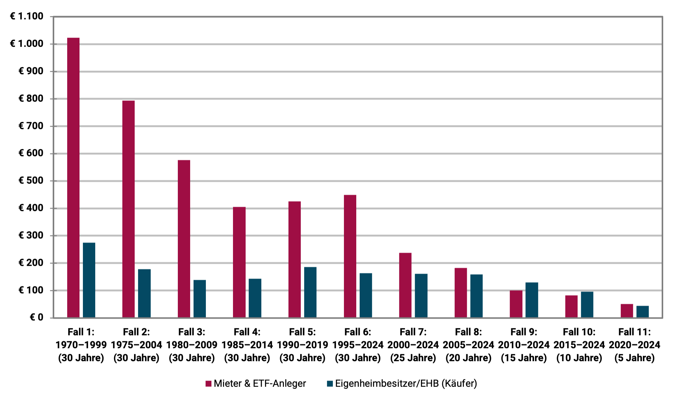
► Final assets in EUR thousand.

The interpretation of the results in the figure: Why is the tenant in the lead in the majority?

In nine out of eleven cases, the tenant/ETF investor achieved a higher final net worth at the end of the second period under consideration. Only in the two cases 9 and 10 is it the other way around. However, the EHB advantage in absolute monetary units is small in these two cases: only 19 and 14 thousand euros, respectively.

In general, cases 10 and 11 have to be classified as less important for our conclusions compared to cases 1 to 9. Firstly because they only represent relatively short periods of time and secondly because of the rather insignificant absolute differences in final wealth between EHB and tenant. One could therefore speak of “draws” in “yield races” 10 and 11. A clearer result in one direction or the other would probably only emerge after another five to ten years.

The main reason why the tenant + ETF investor wins our buy or rent race nine out of eleven comparisons is that the equity global asset class produces noticeably higher total returns in the long term than the residential real estate asset class. This applies to German residential properties and it also applies to other countries for which corresponding total return data for residential properties is available. Nevertheless, it must be noted that residential property returns in Germany have been particularly low compared to other countries since 1970 to the present day.

But why is the tenant's final asset advantage in cases 1 to 6 so spectacularly high? (In case 1, for example, 748 thousand euros in favor of the tenant.) There are four reasons for this.
 
Cause #1: Cases 1 to 6 last the full 30 years, cases 7 to 11 do not. Due to the compound interest effect, differences in returns between two investments A and B have a greater impact on the final assets, the longer the observation period is.
 
Cause No. 2: German residential real estate recorded disastrously low increases in value in the 44 years from 1970 to 2013. At the end of these four and a half decades, the average German residential property, adjusted for inflation, was worth 16% less than at the beginning - the worst value among around 20 western countries for which such data is available.
 
Cause No. 3: From 1970 to 2013, real estate loan interest rates were significantly higher at an average of 7.4% p.a. than from 2014 to today at 2.2% p.a.
 
Cause No. 4: Rents and rent increases in Germany were comparatively low from 1970 to around 2015. During this time, this also favored the tenant/ETF investor side (as did causes 1 to 3).

What influence does the amount of the loan share, the “credit leverage” have?

In our calculation for the illustration, we assumed an initial loan financing of 70% for the EHB. If 100% equity financing had been used (i.e. zero credit), nine of the eleven time window cases would still have been in favor of the tenant, although the distribution of winners and losers and the absolute final asset values ​​would have shifted.

A higher credit percentage than 70%, e.g. B. 85% would also have coincidentally resulted in a 9-to-2 overall result in favor of the tenant as shown in the figure, while this modification would in turn have changed the specific winner-loser distribution across the eleven cases.

In general, it can be concluded that it is popular in the real estate fan community Credit leverage [2] On balance, the EHB was rather detrimental to returns. The lack of financial benefit of the credit leverage effect on the final assets and return on equity of real estate investments contradicts the prevailing opinion in the real estate fan community and among those who make money from selling and financing real estate, i.e. brokers, banks and real estate coaches. In our separate blog post “The credit leverage myth in real estate” we show that and why loan financing (leverage) in commercial real estate financing - where there is better data regarding the effect of debt financing - is statistically detrimental to returns.

What impact would variable loan interest rates have had?

In many Western countries, private real estate loans mostly have variable interest rates, while in Germany long-term fixed interest rates of ten years or more dominate. Would variable interest rates have significantly changed the results in the figure? The short answer: Only marginally and more in the tenant's favor. He would have won the final wealth race in the case of variable interest rates in ten out of the eleven cases. Reason: The interest rates, which have risen sharply since the beginning of 2022, had a less favorable effect on the EHB.

Why does the media regularly report that homeowners are, on average, richer than renters in old age?

How do our results fit in with the statement that has been made repeatedly by the real estate industry, journalists and real estate influencers for decades, that pensioner households that own their own home have, on average, higher wealth than corresponding renter households? On the surface, the statement in question is true, but it is still a case of “lying with statistics”. For these households, home ownership is not the cause of their higher wealth, but rather the consequence - more precisely, the consequence of higher income, typically over decades, combined with a permanently higher propensity to save. [3] In addition, there is a statistically larger and/or earlier increase in assets through donations or inheritances for EHB households relative to tenant households.

Here is an illustration of the real estate industry's manipulative swapping of cause and effect in the situation just described: The average wealth of all Ferrari-owning households in Germany naturally exceeds that of non-Ferrari owners. Now the question: Was the Ferrari the cause of this wealth advantage? Of course not. If anything, the Ferrari did damage. Either way, the Ferrari ownership was the result of the wealth advantage. It's the same with home ownership. He is the one Consequence the above-mentioned causes (primarily higher income, higher propensity to save and therefore higher wealth). If one were to compare renters with homeowners who had the same long-term income and the same propensity to save, and if inheritance effects were taken into account, it would be shown that renters statistically achieve higher final wealth in retirement. However, such empirical studies do not exist for Germany.

What about the home ownership advantage of the “positive compulsory savings contract”?

Earlier we mentioned the higher propensity to save among home-owning households. A higher propensity to save can have two causes: (a) A higher income. It falls e.g. B. It is easier to save 20% of 10,000 euros of net income per month than 20% of 2,000 euros. Furthermore, the absolute savings amount in the former case is 2,000 euros and in the latter case only 400. (b) A purely psychologically caused higher “savings affinity”, i.e. if two households A and B have an identical net income, but household A saves 30% of it and household B only 5%, then household A has a purely psychologically caused higher propensity to save. In plain English: Household A is more economical and cuts down on consumption more.

If a home is financed with debt with a debt ratio of around 60% or higher, then this household will have to incur higher real estate-related expenses per month from loan annuity and other real estate expenses (average maintenance, insurance, property tax) than a comparable renter household. This difference exists until the annuity loan is fully repaid, usually 25+ years. Now the crux of the matter: Such an EHB household has no choice in making these expenses month after month until the loan has been fully repaid, otherwise it would lose the property to the bank through a seizure and would also perceive this loss as a social stigma. The comparable tenant household, however, is not under such pressure and risk with its ETF savings plan. He can stop saving every month and instead consume more without any short-term negative consequences. The tenant therefore needs a good deal of self-discipline in order to spend the same amount every month on financial training as the EHB for 25+ years. The latter, on the other hand, “is forced to do so by the circumstances” and is subject to a “positive compulsory savings contract” because of his real estate loan.

This effect - which is nothing other than the statistically higher propensity to save among owner-occupier households mentioned above - contributes to the fact that EHB households are actually statistically wealthier in old age than renters. But again: the statistical asset advantage of EHBs has nothing to do with the high profitability of the property. If anything, it can be said that this asset advantage despite of the home, not because of it. If a renter household has the same saving discipline as a home-owning household, the renter household will statistically have achieved a higher and often significantly higher final wealth by the age of 50, 60 or 70.

What if you don't use a 100/0 stock portfolio for the tenant, but rather a 60/40 stock-bond portfolio?

We based our rent-versus-buy comparison with a tenant on a 100% equity portfolio (an MSCI World ETF) because we believe that a globally diversified equity ETF on a buy-and-hold basis is less risky than a debt-financed investment in a single property. [4] (The fact that it is easier to observe and measure the ongoing fluctuations in the value of an ETF portfolio than the ongoing fluctuations in the value of the equity position in an individual property does not change this basic fact.)

If the tenant were to be based on a 60/40 portfolio consisting of an MSCI World ETF and a bond ETF (medium-term high-quality bonds), the final asset race in the eleven cases would no longer be 9 to 2 for the tenant, but only 7 to 4. The change in the result illustrates what we all ultimately know: stocks produce far higher returns in the long term than interest-bearing investments.

Two biases in favor of homeownership in our calculations

In two ways, our buy-or-rent calculation is biased in favor of buying.

Aspect 1: The calculation assumes that only one property purchase takes place during the observation periods. Although there is no data on the average holding period (median holding period) of a home in Germany, it is likely to be less than 30 years. Such figures are available for the USA. There, the median holding period for a home is around twelve years. In Germany it will be longer, but probably shorter than 30 years. Due to the very high transaction costs (additional costs of buying and selling) in real estate, the return on a home decreases as the holding period decreases. In addition, if a loan-financed home is sold “early,” there may be an expensive prepayment penalty on the loan.

Aspect 2: When taxing the tenant's stock ETF portfolio, the tax advantage that buy-and-hold has under the German withholding tax was not taken into account. We quantified this tax advantage in a separate blog post (“Save taxes through buy-and-hold”).

The academic literature on buying versus renting

Our buy-or-rent results for Germany presented here are consistent with the basic trend from a number of similar historical buy-or-rent studies or general real estate yield studies for other countries and time periods. At the end of this blog post we list 18 such academic studies in the appendix under point 3.

Conclusion

In the 55 years from 1970 to 2024, renting combined with a simple, broadly diversified stock investment on a buy-and-hold basis was statistically more profitable in Germany than buying a home. This is what our empirical calculation shows and which is confirmed by a large number of comparable analyzes by researchers for other countries and time periods.

These results contradict what most Germans believe about the relative economic attractiveness of buying or renting.

The fact that banks, brokers and real estate influencers claim otherwise can easily be explained by the conflicts of interest of these parties.

The fact that many journalists and media outlets have been repeating the “buying is predominantly more profitable than renting lie” for decades is probably the combined result of “parroting prevailing opinions” and “not wanting to do strenuous research”. In addition, the mainstream media is reluctant to mess with wealthy advertising customers from the real estate and banking industries.

Attachment

Appendix (1): Free Buy or Rent Calculators on the Internet (in alphabetical order)

• Financial flow, independent finfluencer
• Financial tip, consumer protection organization (non-profit)
• Frankfurter Allgemeine Zeitung (daily newspaper)
• Gerd Kommer, author, asset manager (that “Buy versus rent tool” for the book “Buy or rent” by GK can be downloaded free of charge as an Excel file from Campus Verlag under the menu item “Additional material”)
• fmh financial advice, real estate portal (owner: private individuals)
• immoscout24, real estate portal (owner: Scout24 SE)
• real estate world, real estate portal (owner: Axel-Springer-Verlag)
• Dr. Small, credit broker (owner: Hypoport AG)
• Lazy Investors, independent finfluencers
• Stiftung Warentest, consumer protection organization (owner: non-profit foundation)

Appendix (2): The assumptions and data used in the calculation in the figure/graphic

On the real estate side (homeowner/buyer): The property costs 100,000 euros in all eleven cases. (For reasons of simplicity, we use the unrealistically low purchase price of 100,000 euros for a home today, but not in the 1970s, in order to calculate with “round numbers”. If one were to assume 400,000 or one million euros instead, for example, this would have no influence on the relative final result.) The additional costs of the purchase (including property transfer tax) are assumed to be 8%, those of the sale to 8% 1.7%. [5] The purchase and additional purchase costs are financed 30% from equity and 70% from a loan. The loan interest rates are the interest rates for annuity loans to private households with a ten-year fixed interest rate (the interest rate is adjusted every ten years). It is assumed that it will take 30 years for full repayment. The increase in value of the property corresponds to that of the average German residential property during this period. The ongoing additional costs (maintenance, insurance, property tax) correspond to 1.3% p.a. of the current property value. [6] The underlying statistical data comes from the BIS Basel and Bundesbank websites.

On the tenant side (tenant + ETF investor): The tenant initially invests the equity share of 32,400 euros initially spent by the EHB in a world portfolio consisting of an MSCI World index fund (ETF), as such a portfolio is comparable to a debt-financed individual property in terms of its long-term risk. Assumedly he lives in an identical property as the EHB. The rent for this property is based on the historical rental yields for residential properties (apartments) in Germany. Since the tenant's monthly or annual rent is below the EHB's total cash outflow, the tenant saves the difference every month in his ETF portfolio, so that both always spend the same amount on housing and wealth creation. The underlying statistical market data comes from Bulwiengesa and MSCI.

At the end of each of the eleven cases/periods under consideration, both EHB and tenants sell their investments. The tenant pays tax on his ETF investment continuously (dividends) and at the end when it is sold (price gains). Price gains from stock investments were tax-free for private investors in Germany until the end of 2008, after which they will be subject to capital gains tax. [7] Capital gains on homes are tax-free in Germany. In the five cases 7 to 11, the observation period is shorter than 30 years. Therefore, you will have a remaining debt balance with the EHB at the end of the period. To simplify matters, we assume that it will be repaid from the property sale proceeds without any early repayment penalty.

The payments (initial equity deposit and subsequent payments) for the buyer and tenant for the eleven cases are as follows. Case 1: €333 thousand, Case 2: €306 thousand, Case 3: €313 thousand, Case 4: €279 thousand, Case 5: €281 thousand, Case 6: €245 thousand, Case 7: €212 thousand, Case 8: €160 thousand, case 9: 119 thousand euros, case 10: 84 thousand euros, case 11: 54 thousand euros. (Cases 1 to 6 have the same length and should therefore have approximately the same amount of deposits. The existing differences result from different interest levels.)

Appendix (3): List of scientific studies on empirical comparisons of returns from buying or renting

The studies mentioned in the following table come to the conclusion for different time periods and countries that either real estate has lower total returns than stocks or that renting + capital market investment is overall more profitable than purchasing a home with or without debt financing.

Scientific studies on historical returns on residential properties or on buy-or-rent comparisons for different countries or major cities and different time periods

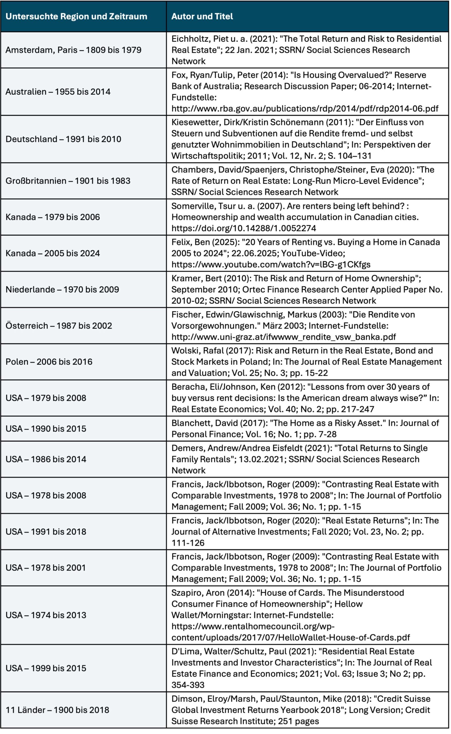
► This literature evaluation primarily took into account scientific studies that cover sufficiently long historical periods, as periods of less than approximately 25 years are only of limited or no significance. ► Not taken into account were (a) publications from the banking or real estate industry that were obviously burdened by conflicts of interest; (b) studies that represent only long-term historical appreciation rather than total returns on residential real estate; (c) buy-or-rent studies that formulate purely model theoretical conditions under which either buying or renting is more attractive; (d) Forward-looking, purely predictive buy-or-rent analyses.

Endnotes

[1] In the 1970s, index funds/ETFs were not yet available for private investors in Germany, but even then a private investor could have easily acquired a broadly diversified stock portfolio on a buy-and-hold basis.
[2] “Credit leverage” = The effect of partial debt financing on the return on equity of an investment (leverage effect).
[3] The propensity to save means the percentage of a household's net income that it does not consume, i.e. invests in wealth creation.
[4] If the property is at construction risk (in the case of a new build or major renovation), the property is even riskier.
[5] The sum of these transaction costs is likely to be at the lower end of what is usual in the market.
[6] In our separate blog post “Maintenance costs – how to calculate real estate investments” let's make this assumption plausible.
[7] We did not take into account the fact that price gains from so-called “old cases” – ETF shares that were acquired up to the end of 2008 – remained tax-free to a limited extent even after 2008, to the detriment of the tenant.

The post Renting or buying – which is more financially attractive? appeared first on Gerd Kommer.

In a YouTube video by British finance professor Patrick Boyle about the current crisis in the UK commercial real estate market, Boyle says "No-one loves leverage more than real estate investors" [1] (Video link here). In fact, the crisis in the commercial real estate market in the UK, Germany, USA and other countries since 2022 has a lot to do with too much debt in the commercial real estate sector. Boyle's sarcastic remark about the popularity of debt financing and the credit leverage effect among real estate investors is correct. To illustrate this, here are relevant statements from German real estate finfluencers: [2]

• “Use as little equity as possible” – chapter title in an advice book on investing in residential real estate by Florian Roski and Mario Geiss
• “You won’t get rich without debt” – real estate finfluencer Tobias Claessens in a LinkedIn post from October 2023
• "Building wealth through real estate is possible for everyone. Even for you, without a lot of equity." – Title of a TikTok video from March 2024 by real estate finfluencer “Immo-Tommy” [3]
• “The leverage effect makes real estate investors really rich!” Title of a marketing video on the real estate agent's website Bartz Real Estate

In this blog post we would like to show that the leverage effect in real estate investments is presented alarmingly uncritically by many representatives of the real estate industry, including brokers, property developers, real estate finfluencers, providers of courses on investing in real estate (“real estate coaches”) and authors of advice books in the “Get rich with real estate” category.

We believe this primarily because there is simply no scientific or otherwise objective, hard evidence and figures that show that the credit leverage effect in real estate financing has even a somewhat reliably beneficial effect.

This is the result of our evaluation of the specialist literature from authors without conflict of interest on the effect of leverage in real estate investments. This involves both professional commercial investors and investments by private households - small landlords [4] and owner-occupiers. In Appendix 1 at the end of this article, we list a dozen specialist articles that show that a high proportion of debt capital in commercial and private real estate investments statistically has no financial advantage or is even detrimental to returns, i.e. it worsens either the absolute return on equity or at least the risk-weighted return on equity. The risk of real estate investments (in contrast to their return) always increases through leverage anyway.

As far as we know, there are no independent academic studies on the historically realized returns on equity of small landlords in Germany - with one exception: a study by the German Institute for Economic Research (DIW) from 2014 for the period from 2002 to 2012. With regard to the equity returns achieved by landlord households, this analysis comes to sobering results for small landlords. We have them here summarized in a previous blog post on rental property returns (link to original study here).

For homeowners in Germany, leverage has reduced returns in most long-term time frames over the 54 years since 1970. [5] This is based on figures in Kommer's book Buy or rent presented and more condensed in a blog post (here). Similar results were also found in other countries such as Australia, the United Kingdom, the United States and the Netherlands. Historically, the combination of rents and passive buy-and-hold capital market investments in Germany led to higher final wealth in the majority of cases. And the financial disadvantage of buying compared to renting + capital market investment tended to be greater the more borrowed capital the buyer used to finance his home.

A previous blog post of ours entitled “Leverage stock investments with credit – does it work?” (see here) contains a list of scientific analyzes that show that leverage in companies generally - not specifically in real estate companies - has a statistically negative impact on shareholder returns or company operating returns.

So if there is no hard numerical evidence that leverage has a reasonably reliably positive effect on the returns on equity of real estate investors and companies outside the real estate sector, why are brokers, real estate finfluencers, real estate coaches and the many authors of “get rich with real estate books” the majority of ardent advocates of credit leverage?

The answer to this question should not surprise anyone: The real estate service providers mentioned benefit from the highest possible number of small landlords and owner-occupiers in their business who believe that (a) you can get rich quickly with real estate, (b) that you can do this with little equity and (c) that the additional risk associated with borrowing is not too high.

How does the real estate industry convince private households of the attractiveness of “get rich by buying real estate on credit”, even though there is obviously no hard statistical evidence of success for this? This can be done by real estate service providers using one or more of the following six marketing tricks in their marketing. All six have the direct or indirect purpose of using credit leverage as a “magic tool”, [6] as a species Free Lunch when investing in real estate with little or no equity.

Marketing trick 1: Calculate the credit leverage effect

Almost inevitably, a calculation example similar to the following is presented in publications by those who earn directly or indirectly from the sale of loan-financed real estate. These calculations, which are “funny” from a technical perspective, could be titled “Getting Rich on an Excel Sheet”.

Figure 1: Weird example calculation of the credit leverage effect on a real estate investment in “Year 1”

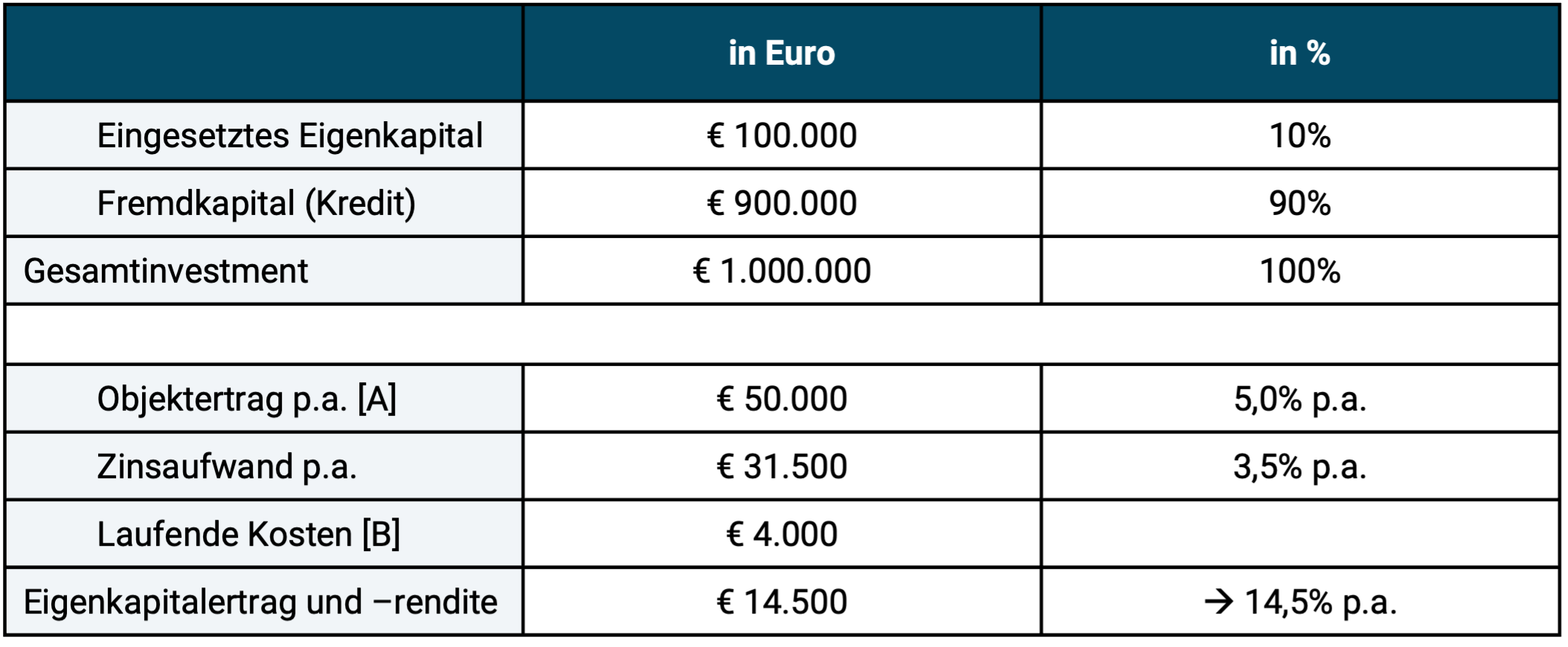
► [A] “Property income” is defined here as gross rent plus increase in value. ► [B] Maintenance, insurance, property tax. 4,000 euros is at the upper end of what the real estate industry would typically state as a percentage, but is still clearly too low. ► The calculated percentage equity return is 14,500 ÷ 100,000 = 14.5%.

Extended calculation examples of the credit leverage effect such as the one in Figure 1 are intended to show that even with relatively low returns from residential real estate investments (net rents and increases in value [7]) attractive double-digit returns on equity result. [8]

You don't have to take such coaster calculations on the leverage effect seriously - not even if you accept that they are intended "for illustration purposes only". They are not to be taken seriously because they are deliberately created from a purely “accounting” perspective, which is ultimately incomplete. If they were complete, they would first of all have to be on one Cash flow basis or “internal rate of return basis”. However, this includes the cash outflow for loan repayment. With small landlords, repayment can never be avoided in the long term - even less so with owner-occupiers. [9] If one were to simplify the example in Figure 1 and take into account a linear loan repayment over 25 years (4% per year = 36,000 euros), the return on equity for the period under consideration would no longer be plus 14.5%, but minus 21.5% (loss of 21,500 euros), since interest expenses and repayment together add up to 67,500 euros.

However, omitting repayment does not mean that the credit leverage wizards' bag of tricks has been exhausted.

In other fables about the "magic of leverage" or about "paying for the property with other people's money and then watching it pay off through the rental income" the loan repayment is included, but in return one or more of the following "tricks" is used: The setting of (a) unrealistically high rental yields (the ratio of rents to acquisition costs or market value), (b) unrealistically low maintenance and management costs (in this blog post more on the assessment of the level of realistic maintenance costs for real estate) or (c) it is simply ignored that with such a “self-paying investment” it takes 20+ years until the cash flow for the investor turns significantly into positive territory because only then does the repayment element no longer apply. In other words, 20 long years to achieve “passive income”.

With the exception of interest rates, the inputs for such calculations are rarely from objective statistics and databases and one conservative Interpretation of the real market conditions derived. They are typically optimistic best-case assumptions for advertising purposes.

Marketing trick 2: Tell the old story of rags to (real estate) millionaire

Many real estate agents and almost every real estate finfluencer or real estate coach have them in their marketing repertoire because they are well received by the public: “Exciting stories” about individual investors who have become “financially independent,” “financially free” or “rich” by purchasing real estate with aggressive leverage – i.e. little equity or even no equity at all – and now live on their “passive income”. In order to make these “rags to real estate millionaire” stories credible, they often contain specific names and often even photos of “successful” real estate investors “who made it at a young age”. It is not uncommon for the narrator himself to be the subject of such a “success story” à la “how I got rich with real estate – and you can do it too!” Because of their specificity (names, photos), the stories seem credible to many recipients.

The unfortunate thing is that this anecdotal evidence can never be verified by outsiders. The majority of these descriptions are likely to be manipulated and some are completely made up.

In addition, the assets of the “successful” real estate investors stated in the stories are almost always properly inflated. In the “personal success story” the property value or the number of properties of the investor is mentioned: “Sebastian already owns nine properties at the age of 29” or “Lisa has a real estate portfolio worth seven million euros after five years”. There is always no information about the debts. [10] This is important because in every other industry outside of real estate and in life in general, “assets”, “wealth” or “net worth” are always referred to as Netassets are stated and understood, i.e. as gross assets minus debts. The general 2,000-year-old rule that “wealth” is the value of all of a person’s (or company’s) assets minus their debts (i.e. equity) applies everywhere except in the real estate industry.

Marketing Trick 3: Repeating the “Inflation will devalue your loan debt” myth

The spread of this “theory” is particularly useful for those who have little capital but want to finally become “rich” because it simply sounds too tempting: “Accrue debt that you only have to pay back in part!” And because this “theory” sounds smart and logical when quickly explained by the “financial experts”, it is believed by probably 90% of those who hear it.

The voodoo logic goes like this: Credit borrowers receive a financial advantage through inflation because their income (e.g. rents collected or their own salary) increases in the long term with inflation, while the amount of their debts and (in the case of fixed interest rates) the interest element are fixed. Both should therefore become less and less or “devalued” over time, adjusted for inflation (in real terms). This makes debts easier to service and pay off from year to year. But this apparently plausible thinking is only half the truth, and in this case the half truth is a complete lie.

The missing half of the economic reality in such fantasy stories: Due to inflation, nominal interest rates are higher than they would be without inflation. Inflation only devalues ​​what the market inflation expectations previously added to the debt service (interest + repayment). We have explained what these economic connections look like in detail in a separate blog post (here). For reasons of space, we will therefore not specifically refute the inflation-devaluation-debt fiction in detail here.

Marketing trick 4: Hide hard figures on the German real estate market

In no other country for which long-term data on increases in the value of residential property are available have these been as low as in Germany since 1970. The increase in the value of residential real estate in this country, adjusted for inflation, averaged 0.1% p.a. from 1970 to 2023 (54 years). The average German residential property was worth a paltry 7% more in real terms at the end of 2023 than 54 years earlier at the beginning of 1970. Even in Japan, residential property prices rose faster. We have this fact, well known among experts here (blog post) and here (YouTube video) documented.

Yes, in the time window from 2010 to 2021 (12 years), the increases in the value of residential properties in Germany were very high. They were that because they were particularly low in the previous 40 years from 1970 to 2009, namely an average of minus 0.4% p.a. in real terms. Due to this return disaster, residential property prices in Germany were 16% below the 1970 level in real terms at the end of 2009. Because of their exorbitantly low valuation in 2009 compared to international standards and interest rates continuing to fall at the time, German residential property prices began to fall at the beginning of 2010 for twelve years until the end to rise sharply in 2021. Since 2022 they have fallen again and in September 2024, adjusted for inflation, they were 17% lower across Germany for existing properties than in February 2022. Ergo: The twelve years from 2010 to 2021 were a positive outlier against the long-term trend that was not representative of the long-term future.

Of course, increases in value are not the total return of a real estate investment, but if the real increases in value are close to zero in the long term, the statistical chances of high leveraged returns on equity are not good from the start.

Occasionally, in this context, one comes across the truly famous statement from some chronic real estate optimists:the There is no real estate market, every property is an individual case." If that were true, then there would be the stock market, the bond market, the raw materials market or the Not the automotive market. There would then actually be no market, just individual investments. Funny! The fact is that the prices of probably over 80% of all individual properties in a city or region correlate highly with the general price trend in the corresponding area and in the minority of properties for which this was not the case in retrospect, we knew it ex ante usually none.

Marketing trick 5: Present real estate as a particularly safe investment class

We have all heard it countless times in our lives from our grandparents, from real estate agents, real estate influencers, bankers, tax advisors and from our buddy who has just bought a condominium: residential properties are “particularly safe” investments. The Sparkasse Pforzheim Calw (Baden) puts it almost comically and bordering on unintentional satire in a marketing publication that is no longer available: “Real estate, probably the safest investment in the world […] Real estate has been one of the safest, most stable investments in Germany for decades - and it will maintain this status.”

However, the reality shines less than the dusty cliché of “stable concrete gold”. Housing prices can crash - just like stock prices, long-term bonds, high-yield bonds, the price of gold, Bitcoin or a private equity investment. However, a crash in real estate usually (but by no means always) occurs more slowly than in stocks and is therefore often not perceived as a crash.

Some crash examples of the decline or collapse of residential property prices (all figures adjusted for inflation): USA over six years from 2006 to 2011: minus 39%, Ireland over seven years from 2007 to 2013: minus 57%, Netherlands over eight years from 1978 to 1985: minus 51%, Japan over 20 years from 1990 to 2009: minus 49%, Germany over 30 years from 1981 to 2010: minus 31%.

In every country in the world for which data of sufficient quality and length is available, there have been declines in the national real estate market over the past 100 years that exceeded 30% in real terms. In France, real property prices fell cumulatively by 84% from 1911 to 1948. It then took the price level another 15 years to return to the level of 1911. Main cause: economic problems in the context of the First and Second World Wars as well as rent controls introduced in 1911, which were only gradually relaxed around 1948.

All of these numbers (a) exclude the loss-increasing effect of leverage and (b) all of the numbers refer to entire national markets. This means that half of all individual properties in these markets performed even worse, and the possible downside is even more extreme than is reflected in these market averages without leverage and transaction costs.

You rarely or never hear statistical data on past slumps in the residential real estate market from credit leverage advocates.

Compare the real estate industry's silence regarding historic droughts and slumps in the real estate market with the situation with equity investments, bonds, raw materials, gold or cryptocurrencies and the financial products derived from these asset classes. Inflation-adjusted historical long-term data, including drawdowns, crashes and duration of recovery phases, are freely available there and have long since been swept under the table by the industry. The reason they won't do this is because anyone who would do so would rightly be seen as a fool or a rip-off. With regard to the “stock crash of the century” from 1929 onwards, the collapse is even regularly overstated (see here).

Anyone who has ever bought a share or a share ETF anywhere in Germany in the last 20 years will inevitably have to click through or literally wade through risk warnings such as “there are high risks associated with investments in securities, including the risk of total loss” before making the purchase. This is transparency and realism.

Of course, total losses are also possible with credit-leveraged real estate investments, especially in severe market crises and in the case of individual unfortunate transactions even in good market phases. Nevertheless, one hears very little about evidence of such risk of loss in credit-financed transactions in the real estate industry and if there are, then they were “isolated cases” or “special cases”.

Marketing Trick 6: Statistics mean nothing because a smart investor only focuses on the best deals

It is the most widespread and probably the oldest of all real estate marketing tricks. It is mainly used when the previous five did not achieve the goal. The trick is the “brilliant” observation that statistics, empirical data and the usual factual logic do not have to apply “if you specifically select particularly financially attractive deals”. With the superior know-how that the respective advice book author or real estate coach imparts, in combination with the “commitment” and “focus” of the investor, this is of course not a problem. This brings to mind the advice of the American comedian Will Rogers (1879 - 1935) on successful investing in stocks: "Don't gamble. Take all your savings and buy some good stock and hold it until it goes up, then sell it. If it doesn't go up, don't buy it." [11] Further comments are unnecessary.

What are rational, sensible reasons for debt-financed investing in real estate?

Of course, there are rational reasons for using debt capital to finance real estate. These include, for example, these two:

• For property for personal use: Without external financing, a typical household would only be able to purchase a home at the end of their working life or even later. Here, debts serve to bring forward “consumption” over time. Bringing forward a consumption or investment decision has been the essential purpose of debt for 3,000 years, not exploiting the credit leverage effect.
• For small rentals: Debt-financed investing and credit leverage can have a positive effect for an investor (a) if he is 100% clear about the considerable risk of leveraged investments and has analyzed its economic and legal consequences thoroughly and competently, (b) if he knows that with fewer than around six to ten residential units the economic logic works pretty mercilessly against him, (c) if he reduces the level of debt to a more moderate level as the company grows and succeeds, lowered to a lower risk level [12] and (d) if he obtains legal notice at the earliest opportunity Firewall between commercial debts on the one hand and his private assets on the other. This means that he then holds a sufficient amount of wealth in the private sphere. With these private assets, he is no longer liable for investment liabilities. But these private assets that have been brought into the security zone can of course no longer be leveraged.

Conclusion

As we have shown here, the impact of credit leverage is naively and optimistically portrayed by much of the real estate industry.

According to academic studies, leverage appears to statistically worsen rather than improve the absolute return on equity or risk-weighted return for large commercial real estate investors, small landlords and owner-occupiers. Even outside the real estate industry, corporate debt statistically has a negative impact on key business metrics or shareholder returns.

Of course, someone who bought a residential property in Germany between approximately 2005 and 2018 and financed a significant portion of the purchase price with debt will have achieved excellent returns on equity after a holding period of five to ten years or more [13] – provided there was no isolated case of bad luck or inability. However, things looked less positive for purchases well outside this time window.

Against this background, the obsession with leverage in much of the commercial real estate sector, as reflected in Patrick Boyle's quoted statement at the beginning of the undying love between real estate and credit leverage, is highly ambivalent. However, it is clear why it exists: without leverage there would be fewer transactions for real estate service providers and therefore less money. And without accepting high leverage, a naive but important dream for many young people would collapse: “Get rich quickly without equity”.

It is high time that the real estate industry, financial journalists and finfluencers practice more honest, evidence-based communication about credit leverage.

Endnotes

[1] Leverage, Leveraging = credit leverage (effect), debt; Lever = lever.

[2] Social media influencers who specialize in the topic of money and wealth.

[3] Over Realty Tommy - according to their own statements, Europe's largest real estate finfluencer - Spiegel and NDR have published several articles and videos about Immo-Tommy's supposedly unfair business practices since August 2024. At the moment (as of November 2024) it is unclear how the matter will turn out for him.

[4] “Small landlord” is the terminology used by the Federal Statistical Office. This refers to landlords who do not operate the rental business full-time (non-commercially), usually with fewer than six to eight residential units.

[5] “Since 1970” because there is sufficiently good data available from that year onwards. How leverage worked beforehand is more difficult to assess due to a lack of sufficiently granular raw data.

[6] Quote from the book “10x for real estate investors – achieve more, grow faster, increase your portfolio tenfold” by Markus Beforth (2024).

[7] Net rent = gross rent less expenses for (average) maintenance, property tax and insurance.

[8] At the end of this blog post there is an Appendix 2 with a more detailed explanation of the leverage effect. Readers who are not yet well acquainted with the mechanics of debt capital leverage can find out more about this in the appendix.

[9] There is a fundamental difference here to large commercial landlords, where the banks accept that there is a permanently constant level of debt at the company level and that there is therefore no net repayment at the portfolio level. This is one of the many structural advantages of large investors relative to small landlords.

[10] For the sake of completeness, it should be mentioned that the numerical information on objects and object values ​​cannot be checked here either. Why should these unverifiable numbers be true if they are obviously for marketing purposes?

[11] "Don't gamble. Take all your savings and buy a good stock. Hold it until it goes up. Then sell it. If the stock doesn't go up, don't buy it."

[12] If René Benko (Signa-Immobilien) had observed this simple risk management principle, he would not now be bankrupt and socially ostracized.

[13] Because the period mentioned includes all or most of the “golden German real estate era” from 2010 to 2021 as well as the zero interest period from 2016 to 2021.

Appendix 1

Below is a list of specialist articles that show that high leverage in commercial and private real estate investments tends to lower the absolute return on equity or the risk-weighted return on equity.

(a) Commercial real estate investments

Alcock, Jamie et al. (2013): “The Role of Financial Leverage in the Performance of Private Equity Real Estate Funds”; In: Journal of Portfolio Management; 39; No. 5; 2013, internet source here

Case, Brad (2017): “Comparing Listed REITs with Private Equity Real Estate: What the Cambridge Associates Data Have to Say”; Aug 16, 2017; Nareit/National Association of Real Estate Investment Trusts; Internet reference here

Giacomini, Emanuela/David Ling/Andy Naranjo (2016): “REIT Leverage and Return Performance: Keep Your Eye on the Target”; August 17, 2016; SSRN; Internet reference here

Haughwout, Andrew et al. (2011): “Real estate investors, the leverage cycle, and the housing market crisis,” Staff Reports 514, Sept. 2011, Federal Reserve Bank of New York

Pagliari, Joseph (2017): “Another Take on Real Estate’s Role in Mixed-Asset Portfolio Allocations”; In: Real Estate Economics, Volume 45, Issue1, Spring 2017

Green Street Advisors (no author) (2009): “Capital Structure in the REIT Sector”; July 1, 2009; Working Paper; Internet reference here

Sagi, Jacob/Zipei Zhu (2022): “Leverage in Private Equity Real Estate”; March 21, 2022; Working Paper; SSRN; Internet reference here

Thomas, Brad (2012): “REITs With Modest Leverage: Separating The Best From The Rest”; July 02, 2012; Wide Moat Investors; Internet reference here

 
(b) Private/non-commercial real estate investments

Beracha, Eli/Johnson, Ken (2012): “Lessons from over 30 years of buy versus rent decisions: Is the American dream always wise?” In: Real Estate Economics; 2012; 40; No. 2; Internet reference here

D’Lima, Walter/Schultz, Paul (2021): “Residential Real Estate Investments and Investor Characteristics”; In: The Journal of Real Estate Finance and Economics; 2021; 63; Issue 3; No. 2; Internet reference here

Mian, Atif/Amir Sufi (2010): “House Prices, Home Equity-Based Borrowing, and the U.S. Household Leverage Crisis”; April 2010; SSRN; Internet reference here

Jud, Donald/Daniel Winkler (2005): “Returns to Single-Family Owner-Occupied Housing”; Journal of Real Estate Practice and Education; Vol. 8, No. 1; 2005; Internet reference here

Schweizer, Jonas/Alexander Weis (2022): “Buy or rent? – Home vs. global portfolio”; Gerd Kommer Invest; Dec 2022; Internet reference here

Appendix 2: How the credit leverage effect works

First, a case study of how the leverage effect works:

Antonia invests 100,000 euros in an investment project We now imagine two scenarios. In scenario 1, the value of project

What effect does the two scenarios have on the return on Antonia's equity (EK)?

In scenario 1, Antonia's equity return is 30,000 euros ÷ 60,000 euros = plus 50% (profit from equity), in scenario 2 the equity return is -30,000 euros ÷ 60,000 euros = minus 50%. (We ignore the borrowing costs and any tax effects here for the sake of simplicity. Assumedly, there is no loan repayment.)

Without leverage, equity returns would have been plus 30% and minus 30%. (Where there is no leverage, equity return and return on assets, or “property return” in real estate jargon, are the same.)

We see that leverage symmetrically increases both the opportunity (the upside) and the risk (the downside).

In general, leverage results in increased equity returns for a given period, be it six months or 20 years, when the debt expense (absolute or percentage) is lower than the total investment return (absolute or percentage). The general formula for calculating return on equity is:

$\mathrm{EKR}=\mathrm{GKR}+\frac{\mathrm{FKA}}{\mathrm{EKA}}\cdot (\mathrm{GKR}–\mathrm{FKZ})$

Explanation of abbreviations: EKR = return on equity, GKR = return on total capital, FKZ = interest rate on debt capital, FKA = share of debt capital in percent or absolute, EKA = share of equity in percent or absolute.

A numerical example. We use Antonia's investment in scenario 1 and a loan interest rate of 3%: EKR = 30% + (40% ÷ 60%) × (30% - 3%) = 48% (rounded).

With leverage you can also lose more than 100%. A numerical example: Antonia once again invested 100,000 euros in project A using leverage, this time with only 30,000 euros equity and 70,000 euros FK. Now the value of Project A collapses by 40% within a few months. Antonia has now lost her entire equity of 30,000 euros and owes the bank another 10,000 euros. In percentage terms, your loss is –40,000 ÷ 30,000 = –133%

So we have seen that leverage symmetrically increases both upside potential and downside potential.

In an essay in 1958, two American economists, Franco Modigliani and Merton Miller, provided theoretical evidence that corporate leverage does not produce a systematic advantage in terms of risk-weighted return on equity (at least if one ignores possible tax advantages). Modigliani and Merton Miller received the Nobel Prize in Economics in 1985 and 1990, respectively, for this groundbreaking research work (Modigliani, Franco/Merton Miller (1958): “The cost of capital, corporation finance, and the theory of investment”; In: American Economic Review; Vol. 48; 1958).

The post The credit leverage myth in real estate appeared first on Gerd Kommer.

Owner-occupied residential real estate is a popular form of retirement planning. Around 45% of all German households live in their own home (owner-occupied apartment or house). According to surveys, around two thirds of all renter households also want to own their own home in the short or long term.

However, owning a home as an element of retirement provision has a structural disadvantage for many households who are about to end or have already stopped working and who do not fall into the “very rich/very wealthy” category, which we will get to the bottom of in this blog post. (We have dealt with the often overestimated profitability of residential properties and their often underestimated risk in recent years from different perspectives see here and here as well as the list of our blog posts on this at the end of this text.)

The fundamental disadvantage of real estate as an investment in the asset reduction phase

We illustrate the basic problem using the young pensioner household Luisa and Ludwig (hereinafter “L&L” for short). Both are 65 years old and both have just finished their careers. The couple has built up a fortune of 500,000 euros over the last 25 years and is debt-free. After completing their professional activity, L&L have now moved from the asset accumulation phase to the asset utilization phase.

In our first observation scenario - let's call it "Universe A" - we assume that L&L's assets of 500,000 euros consist entirely of liquid assets, namely an ETF portfolio worth 300,000 euros (a single ETF that represents the asset class Stock Global shows) and from an interest-bearing daily money of 200,000 euros. [1] This split or asset allocation is often referred to as a “60/40” portfolio, which usually works well for relatively cautious investing households. The portfolio generates current income (interest, dividends) and price gains in the equity portion.

L&L live in a beautiful three-room apartment for rent. Because their two statutory pensions are noticeably lower than their previous two salaries and they do not want to live a “frugal” life, they now have a combined “pension gap” of 2,500 euros per month or 30,000 euros per year. The two want to cover this gap with their liquid assets, their ETF portfolio and daily money account. The initial “withdrawal rate” is therefore 30,000 ÷ 500,000 euros = 6% per year.

In the case of a liquid investment, as in the case of L&L, this withdrawal rate consists of distributions and share sales in relation to the stock ETF portfolio and of withdrawals in relation to the overnight money account. L&L can flexibly increase or decrease the monthly or annual withdrawal at any time if your actual liquidity needs differ from the plan, which probably happens quite often.

Depending on what average inflation-adjusted (real) return after deduction of costs and taxes is assumed for the entire portfolio, the 500,000 euros would last on average around 24 years until fully consumed with an annual real withdrawal of 30,000 euros, but the exact duration is not significant for the purposes of the matter being analyzed here. [2]

In parallel universe B, we assume that L&L live in a self-occupied three-room apartment, i.e. in their own home. The property has a market value of 500,000 euros. It's the same apartment the two of them live in for rent in Universe A. Again, there are no other assets apart from the statutory pension insurance claims. In Universe B, the two save 16,000 euros a year in living costs due to no rent. [3] Accordingly, their annual pension gap is no longer 30,000 euros, but only 14,000 euros. Now the challenge becomes clear: Where should L&L get these 14,000 euros (around 1,200 euros per month) from if not steal them?

The capital commitment when owning real estate

The problem: The substance or “capital” in a property cannot be used little by little like with a bank deposit or securities account. “Ongoing consumption” is only possible for a property up to the amount of the net rent. The net rent is the (gross) rent less expenses for maintenance, insurance and property tax.

With a home, there is naturally no rental income, but the owner saves expenses equal to the net rent that he would have to pay if the home did not exist. On this point, there is no significant difference between an owner-occupied property and a rented one - in both cases, as an owner, you can only use the current net income, but not the substance tied up in the property, the capital.

Another unfavorable aspect of real estate in the context of liquidity and cash flow: the net rent or net rent saved (as defined above) varies significantly over time from year to year due to the irregularity and "lumpiness" of maintenance expenses. In the case of major repairs, it can even happen in a single year that as an owner you have to put more into the property than you get out of it in the form of the rent saved on your own home or real rent on a rental property. Then there is a negative cash flow. This cannot happen with a securities account (for the often underestimated amount of maintenance costs for residential properties, see here).

According to a lobby organization in the German “real estate annuity industry,” there are said to be over three million homeowners aged 55 and over in Germany who are fundamentally confronted with a liquidity problem due to the capital tied up in their own home, i.e. they have too little liquidity, but at the same time do not want to sell their property (source). The cause of the liquidity problem for these owner-occupier households may be an ongoing pension gap (too little income relative to the cost of living), as in the case of L&L. However, the “money problem” can also result from the desire to modernize the property or finance a larger lifestyle expense (e.g. a camper van or a sailboat).

We will now quickly describe ten financial solution approaches – “liquidity creation models” – for such home ownership households. In nine of the ten approaches, the aim is ultimately to at least partially release the capital tied up in the property for the owners, i.e. to make it liquid, in technical jargon to “monetize” the capital in the property so that it can be used when necessary.

Solution 1: Lower living standards

Basically, this is a non-solution to Luisa and Ludwig's problem and definitely one that they don't want. Furthermore, they see no need to leave an inheritance to their 35-year-old son Louis. Louis earns well himself, married a wealthy woman and has already made it clear that he does not want to inherit anything. Solution 1 is therefore ruled out for L&L.

Solution 2: Selling the home to buy a new, cheaper property

In modern German, this solution is called “downsizing”. However, it is not an option for L&L because they do not want to lower their standard of living. But living in a smaller or less well-located, cheaper apartment would mean exactly that. They are also emotionally attached to their current property.

Solution 3: Selling your home and renting an equivalent property

In this case, L&L would simply sell their apartment and then rent a new, equivalent property nearby. An obvious advantage of the sales solution relative to most other monetization strategies is that this approach is legally and economically very simple. In addition, the new rental property can be selected precisely according to L&L's health-related and other criteria that are important for an older couple at this time, such as accessibility or physical proximity to their son and daughter-in-law.

Solution 4: Rent out part of your home

Bringing in the proverbial “subtenant”: For many reasons, this is not to everyone’s taste and not to L&L’s either. Renting out part of the property also fails in many homes because the property is not suitable for partial rental due to its floor plan or other structural reasons.

Solution 5: Selling the home while granting usufruct rights

The property is sold. The buyer (which could be a specialized company or a private individual) grants the old owner (hereinafter “old ET” for the sake of brevity) a lifelong lease right of usufruct one that is notarized and entered in the land register. In the case of a residential property, this gives the usufructuary (the old ET) the right to continue to live in the property until the end of his life, even though the usufructuary is no longer the owner. [4] The right of usufruct is a centuries-old type of right of use for real estate (or other assets) and is regulated in detail in 59 paragraphs of the German Civil Code (BGB). Because the “encumbrance” recorded in the land register makes the property less valuable for the buyer, the selling price is correspondingly lower relative to a property without usufruct.

The old ET cannot sell, bequeath or give away its usufruct right. Who bears the costs of maintenance can be regulated in individual contracts; typically it is the usufructuary, as he has the full economic benefit from the property.

Instead of a simple purchase price payment, it would also be a lifetime payment Life annuity conceivable that the buyer pays to the old ET (usufructuary). [5] We generally advise against life annuity structures. They have several major disadvantages, including the basic problem that the payer stops paying over the following years or decades, e.g. B. due to bankruptcy. Then the pension recipient can be left out in the cold. This complex risk exists even for large insurance companies such as Allianz and is particularly high for smaller companies or even private individuals. In the case of a home annuity with a life annuity structure, there are instruments to partially reduce this “counterparty risk” (default of the pension payer), for example through a so-called “fallback clause”, but such instruments are at best band-aid solutions and only partially cure the basic problem.

Secondly, life annuities mean an unacceptably high inflation risk for the recipient, as the pension does not increase at all over time or only increases to a small, contractually fixed amount. If inflation was consistently above around three to four percent p.a., the purchasing power of pensions would fall drastically over time. In the event of runaway inflation, almost everything would be gone. [6]

Because life annuities in Germany can only be granted by private individuals, the state and licensed, BaFin-regulated insurance companies, the following “combination model” is often used in practice: Step 1: Purchase price payment by the “annuity provider”, Step 2: Payment of the purchase price into an “immediate annuity” offered by a separate insurance company. (Presumably a commission will then flow from the insurance company to the annuity provider for the placement.)

Either way, from our point of view: stay away from life annuity structures, which in principle can also be used in some of the other real estate annuity models outlined below instead of a simple purchase price payment. In practice, however, life annuity structures are rarely chosen for good reasons.

Solution 6: Sale while granting a right of residence

It is very similar to solution 5, except that instead of a usufruct, a “right of residence” (or, to put it more legally, “right of residence”) for the old ET is entered in the land register. A right of residence is similar to a usufruct, but is more limited under civil law and therefore less economically valuable. For example, a right of residence usually expires worthless as soon as the old ET moves out, which does not apply to a right of usufruct. [7] Because a right of residence is worth less, the purchase price payment to the Alt-ET for a given property, after deducting the burden for the right of residence, is higher than for a right of usufruct.

Solution 7: Partial sale to a specialized financial service provider

If the real estate retirement industry's marketing publications are to be believed, partial sales are the new star in the real estate retirement sky. With a partial sale, part of the home - usually 50%, rarely more - is sold to a specialized financial service provider. This then makes a purchase price payment to the old ET. All of this is notarized and entered in the land register. At the same time, the old ET is granted a lifelong right of usufruct (see comments in solution 5).

In principle, instead of paying the purchase price, a life annuity or a temporary pension (time annuity) is also conceivable, but these pension models are rarely offered in practice due to their legal complexity and economic risks (see again the comments on solution 5).

In the standard configuration, the old ET bears all maintenance costs, including those for the part sold. For the part sold, the Alt-ET has to pay the buyer a monthly “usage fee”, a kind of rent, even though he is not a tenant but a usufructuary. The amount of the usage fee is based primarily on the interest rate at the time of the partial sale and less on the local rent.

In the event of a partial sale, the old ET or its heirs remain involved in the potential for increased value of their share. In a typical partial sales agreement, the Alt-ET can sell the entire property to a third party or its part to the financial service provider at any time. However, under standard industry contracts, the old ET must compensate the financial service provider for any losses and even lost profits at the time of sale (regardless of who it is to) if the property has not experienced a sufficient increase in value since the original partial sale during this “second” final sale. This “value protection clause” in the partial sales contract in favor of the financial service provider is the single biggest disadvantage of the partial sales model. From our point of view, it represents you Deal killer.

Overall, the distribution of opportunities, benefits and costs between Alt-ET and financial service providers in a typical partial sale does not appear to be balanced enough. The German financial regulator BaFin also sees it that way (here).

Solution 8: Rent-back purchase

The sale and leaseback consists of simply selling the property to a private person or to a commercial real estate company. The plan from the outset is to conclude a long-term rental agreement between the old ET and the buyer a “logical second” after the sale has been completed, i.e. to rent the property back to the old ET. Typically, the buyer waives his ordinary right of termination in the rental agreement for a long term or at least for several years, including the right to terminate the lease for personal use. The amount of the future rent can also be bindingly fixed in the long term via a graduated rental agreement or index rental agreement. The new owner becomes the landlord and will bear the future maintenance costs.

In general, the leaseback purchase is legally simple and economically uncomplex. Many normal real estate agents offer the search for a buyer willing to buy back as a service.

Solution 9: Conventional lending on the property (senior citizen loan)

The most obvious solution to monetize a debt-free home that you don't want to sell or move out of is a mortgage, i.e. the "normal" taking out of a bank loan against registration of a mortgage. Because this route is so obvious and legally and economically simple, it is widespread in Anglo-Saxon countries and is even specifically regulated in the USA - expressly for owners over 60 years of age. [8] This process is called there home equity take out, the regulatory-defined loan types “Home Equity Conversion Mortgage” (HECM) or “Home Equity Line of Credit” (HELOC).

But even without its own regulatory framework, the matter in Germany is simple and straightforward: a senior citizen loan (new German “best ager loan”) is an ordinary real estate loan secured by a mortgage. The loan amount is usually limited to 50% of the market value of the property as determined by the bank. The loan, for example, has a term of ten or fifteen years and is “final maturity”, i.e. h. There is deliberately no ongoing repayment. The borrower only pays the current interest. The loan is repaid at the end of the intended term either through a sale of the property, from other means or the loan is extended again.

If an inheritance occurs, the loan can be taken over by the heirs and continued or repaid. If the heirs do not want the property + loan debt (e.g. because the value of the property has fallen below the value of the loan balance), they have the risk-free right to reject the inheritance.

What speaks against lending to monetize a debt-free home? Nothing at all, because it is the simplest and almost always the cheapest solution and probably gives the old ET the least amount of control over their existing home relative to all other alternatives. The old ET remains the owner of the entire object even after the transaction.

Strangely enough, many homeowners in this country believe that (a) taking on new debts at an advanced age is “somehow not right” or (b) that you can no longer get real estate financing from a bank “from the age of 60” - both are wrong. If these two considerations were correct, there would be no widespread home equity take-outs in countries with better developed financial markets than here. Of course, every bank wants and must carry out a credit check before granting a loan, even if the value of the security significantly exceeds the loan amount, as is the case with a best-ager loan. And yes, a borrower household with an average age of 65 needs a certain minimum credit rating, regardless of the security. First and foremost, this means that the pure interest payments (without repayment) can be made from existing liquid assets or current income. But in any case, in our opinion, a household that aims to monetize its home without selling or moving out should first examine the viability of this route.

Solution 10: Borrowing via a “reverse mortgage” (“reverse loan”)

The reverse mortgage (“UH”) comes from the USA like so many financial innovations. There it is called “Reverse Mortgage”. Since it is only offered by a tiny number of financial service providers in Germany and probably all at unattractive conditions, one could almost do without presenting the UH here.

In its standard form, UH works like this: The owner of a debt-free home, usually a retired household, takes out a loan on the property from a bank, which is secured by a first-lien mortgage. However, the bank does not pay out the loan amount to the borrower's household immediately (as with senior citizens' loans), but rather grants them a lifelong monthly pension, a life annuity. The loan debt is still very low at the end of the first month because only a single monthly pension payment has been made. The longer the old ET lives, the more the credit debt builds up. According to the contract, the loan is not repaid during the borrower's lifetime - there is no ongoing repayment and the interest is also "capitalized", i.e. added to the loan debt on a monthly or quarterly basis.

The maximum loan value of the property (the loan amount) is usually 50% of the market value of the property at the start of the transaction. This upper limit and the age of the borrower at the start of the transaction largely determine the amount of the monthly pension payment. The older the borrower is at the start of the transaction (i.e. the lower his remaining life expectancy), the higher the pension will be, other things being equal.

When the borrower dies, the outstanding debts are repaid either by the heirs of the property or (if there are no heirs or they do not want them) through a sale of the property by the bank.

We advise against the UH, especially because it is based on the life annuity model (see solution 5) and is simply too expensive.

It is not uncommon for journalists and representatives of the real estate rental industry to write that UH has not yet become established in Germany, but it is widespread in the USA. That's nonsense. To this day - over 60 years after its invention - reverse mortgages have only been able to gain a measly market share in retirement provision in the USA and are considered a failure in politics and science (see Knaak et al. 2020).

Conclusion

The “home pension” as it is marketed and offered in the German market today is a deceptive package.

It starts with the fact that the real estate retirement industry and its journalistic applause continually use the term “retirement” or “pension” for marketing reasons, [9] but essentially do not offer any financing models that include a pension element.

In our view, the partial sale (solution 7), which is the most common solution in the annuity industry, fails because the distribution of opportunities, risks and costs is unattractive for the existing owner.

The main reasons for the unattractive conditions for partial sales and reverse mortgages are the legal and economic complexity of these constructions and the fact that too many parties on the provider side want to make money: brokers, annuity providers, the annuity provider's bank and, in the case of life annuity models, a life insurance company.

With regard to the partial sale and the reverse mortgage (solution 10), we have explained on a purely factual basis why these two home monetization models are a bad idea. If you don't find our argument convincing and are interested in such a solution, we recommend getting one or, better, several offers. To find providers, the first step is to google “partial home sales providers” or “reverse mortgage providers”. We believe that a concrete offer will confirm our great skepticism in the vast majority of cases.

The sober realization remains that real estate is a structurally illiquid asset. The easiest, fastest, least economically risky, legally secure and cheapest way to get liquidity out of this asset is to sell it. The second cheapest option is conventional lending. However, the monetization effect is more limited when lending than when selling.

As we have shown, selling does not necessarily mean that you have to move out of the property. Selling and not moving out can be done using three proven, uncomplex and legally secure alternatives: selling against usufruct rights, selling against right of residence or rent-back purchase.

For all monetization approaches based on sales or partial sales, it is extremely important that the owner has a valuation report prepared by a professional real estate appraiser before the contract is concluded, who has a sole and exclusive contractual duty of loyalty to the owner and is paid solely by the owner. As a general rule, you should not consider appraisers who have been named or recommended by the seller.

Endnotes

[1] This means that the amount of L&L is within the statutory deposit insurance limit of 100,000 euros per person and bank. Above this limit, bank deposits are not sufficiently secure (see here).

[2] We are talking here about a “real” withdrawal of 30,000 euros, i.e. an amount of money that increases annually from year 1 in line with inflation, so that its purchasing power remains constant over time. But since we are investing with “low” real Calculating returns, we can save ourselves the annual “inflation” of the withdrawal. We have ignored the so-called “return sequence risk” here. If you are interested, you can read our blog post on Monte Carlo simulation (here).

[3] This saving results from a saved annual gross rent of 22,500 euros (for a property value of 500,000 euros, this corresponds to a gross rental yield of 4.5%) reduced by 6,500 euros in ongoing costs per annum for maintenance, insurance and property tax.

[4] In individual cases, a usufruct right can also be limited in time at the request of the contracting parties.

[5] By definition, a life annuity (in contrast to a “time annuity”) flows for life, just like the statutory pension. With a life annuity, the annuity payer is exposed to the “longevity risk” of the annuitant: the longer the annuitant lives, the more expensive it becomes for the annuitant.

[6] In addition to the two main risks and disadvantages of life annuity structures mentioned here, there are others, which we will not go into here for reasons of space.

[7] Housing law is regulated by law primarily in Section 1093 of the German Civil Code (BGB).

[8] The financial markets in the Anglo-Saxon countries (USA, Canada, Great Britain, Australia, New Zealand) are overall more developed, more modern and more efficient than in Germany. Private investor protection is also more strictly regulated there.

[9] For example, “home pension”, “real estate pension”, “stone pension”, “house against pension”, “additional pension from your own home”.

literature

BaFin (without author) (2023): “Partial sale of your property – where are the risks?” – link

Knaak, Peter et al. (2020): “Reverse Mortgages, Financial Inclusion, and Economic Development Potential Benefit and Risks”; World Bank – link

Kommer/Bartosch: “Increases in the value of residential properties – dream and reality” – link

Kommer/Lauterwasser: “Inflation helps me as a borrower – keep dreaming!” – link

Kommer/Schweizer: “Maintenance costs: How to gloss over real estate investments” – link

Kommer/Weis: “Are rental properties attractive investments?”– link

Kommer/Schweizer: “The risk of investing in real estate” – link

Kommer/Schweizer: “The return on investments in real estate” – link

Kommer/Großmann: “Open-ended real estate funds – illusion and reality” – link

Kommer/Bartosch: “Avoid capital consumption: Not a desirable investor goal” – link

The post “Home retirement” – a bad idea appeared first on Gerd Kommer.

The world of investment has probably produced more fairy tales than the two Grimm brothers were able to collect in five decades. One of these fairy tales is the “theory” that real estate service providers and financial journalists have been promoting for decades that inflation is good for borrowers because it “inflates away” the real value of debt. This “theory” is expressed in the following quotes:

"Inflation benefits debtors and harms creditors. Because with the devaluation of money, the real value of claims also shrinks." — Wirtschaftswoche

"Borrowers benefit from high inflation. When the value of money decreases, the debt burden automatically decreases." — The Berlin real estate service provider Living happiness on his website

“As a real estate borrower, you benefit from rising and sustained inflation as the real value of the debt falls.” — The real estate loan broker Dr. Klein Privatkunden AG on his website

“If an inflation rate of 5% lasts for four years, then a fifth to a quarter of your home loan will ‘magically’ disappear.” — New Zealand property services provider OneRoof on its website

“In the event of increased inflation, the loan financing is diluted to the benefit of the borrower because the value of the loan to be repaid loses more value than with normal inflation.” — From the guide book “Practical Guide to Real Estate Acquisition and Real Estate Financing”

The facts look different.

For the majority of all borrowers, inflation has neither a significant positive nor a significant negative effect over the term of their loan. For a minority, inflation is about equally likely to have a financially beneficial or detrimental effect.

Story time in the real estate industry

why this Inflation-is-good-for-borrowers fairy tale from the real estate industry and the media is wrong, we explain below using economic logic and historical data.

The main reason for the lack of veracity in storytime can be summarized as follows: At any given point in time, the inflation expected by the market in the future - the next twelve months or the next 20 years - is already priced into the interest rates on real estate loans (and bonds). To the extent that future inflation is priced into the expense interest, it cannot have a real inflationary effect - whether high or low - because the negative effect on the interest to be paid and the positive effect on the inflation of the balance on which this interest accrues over time cancel each other out.

The inflation expected by the capital market for the future and thus already priced into the expense interest rates and income interest rates can simply be derived from the difference between the current yields on conventional government bonds and inflation-protected government bonds - for any period over the next 30 years. We have the background to this in this one YouTube video and this one explained.

Although it can be off the market ex ante Estimated inflation priced into interest rates for a single year or longer single period may later turn out to be too high or too low, but the market estimate is not systematically too high or too low. It is surprisingly correct on a long-term average – see this YouTube video.

Among economists, the pricing of market inflation expectations into the nominal interest rates of loans or bonds is part of the canon of undisputed basic findings in financial market research.

If the expected future inflation - whether high or low - is already included in the market interest rates and these estimates fluctuate symmetrically on average around the actual inflation rates that will later be realized, then in the long term neither loan borrowers nor bond investors will collectively benefit from inflation. The advantage of paying off the fixed loan from income that increases every year by the inflation rate is offset by the disadvantage that the loan interest is exactly this inflation rate higher than in a world without inflation. Overall and in the long term, the economic essence at the level of all lenders and borrowers is as if there were no inflation at all.

You don't need to be a qualified financial economist with specialist knowledge of the market's inflation expectations to understand this issue - a little common sense will do the trick.

If it were true that borrowers systematically benefited from inflation, then it would also have to be true that lenders were systematically harmed by inflation. Lenders in an economy are primarily banks and institutional investors such as insurance companies and investment funds that invest in loans or bonds. The idea that these professional market participants allow themselves to be ripped off by their debtors worldwide and permanently - this idea seems absurd.

A look at historical data makes the economic logic at work here visible. The following figure shows the development of real estate loan interest rates and inflation in Germany in the 53 years from January 1970 to March 2023.

Figure: Real estate loan interest rates and inflation (CPI) in Germany from January 1970 to March 2023

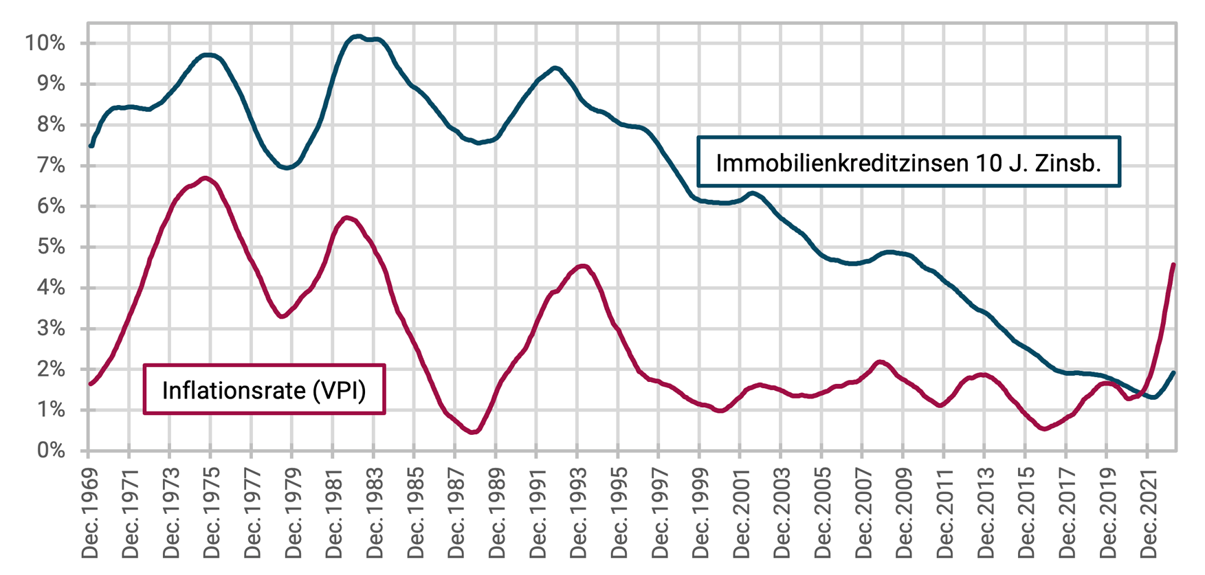
► Interest: German real estate loan interest with a ten-year fixed interest rate. ► Inflation = consumer price inflation. ► In order to smooth the curves and thus make the basic tendencies more visually apparent, the moving average of the previous 36 monthly values ​​is shown for both variables. ► Data: Bundesbank

The graphic shows that real estate loan interest rates and inflation develop quite parallelly in the long term. When inflation rises, loan interest rates tend to rise at the same time; when inflation falls, interest rates tend to fall. The correlation coefficient between the two data series shown here is a relatively high + 0.65.

Individual borrowers can benefit from the fact that loan interest rates and inflation rates do not run exactly in parallel over time, but about the same number of others will suffer a roughly equal financial disadvantage due to the imperfect synchronization. For the majority of all borrowers, there will be neither a serious advantage nor a disadvantage over the entire term of their fixed-rate loan, which usually runs between 20 and 30 years until it is fully repaid and undergoes one or two further interest rate adjustments in between.

A constellation in which the market underestimates subsequent inflation (i.e. initially pricing too little inflation into the loan interest rate) is advantageous for the borrower; a constellation in which inflation is initially overestimated is disadvantageous. In the latter case, the interest burden of such an unlucky person is higher than it would have been if the market had correctly priced in inflation.

Why don't we see the economic logic?

One reason why even financial journalists and many business-savvy people do not understand this financial market logic is that they incorrectly only look at the repayment aspect, i.e. only take into account the beneficial half of the inflation effect. However, its disadvantageous side – the increase in the interest burden – is forgotten or ignored. Of course, this cannot result in a correct overall result.

Whether inflation benefits or harms an individual borrower over the entire term of his loan depends, on the one hand, on the specific historical constellation and, on the other hand, on the length of the interest rate fixation on his loan. Regarding the length of the interest rate fixation: Anyone who takes out a real estate loan with a variable interest rate - the shortest possible interest rate fixation - will very likely have a zero effect from inflation. Anyone who takes out a loan with a ten-year fixed interest rate can either benefit from great inflation-related benefits or suffer great damage.

Since inflation in Germany (as well as most other Western countries) fell trendily and significantly over 40 years from mid-1981 to the end of 2021, one could speculate that most borrowers with long fixed interest rates suffered a financial disadvantage from the actual development of inflation over these four decades.

Galloping inflation or hyperinflation

A special variant of the Inflation-is-good-for-borrowers fairy tale states that runaway inflation or hyperinflation would cause borrowers to lose their debt quickly or even overnight. The fact is that no Western country - where governments are also dependent on the support of the poorer half of the population - will tolerate any significant benefit to property owners due to high inflation.

Let us look at the course of a “historical field test” in Germany, namely the hyperinflation from 1921 to 1923. In fact, it initially led to real estate borrowers at the time being completely relieved of debt in a very short period of time without making any contribution of their own. Salaries, corporate profits and real estate values ​​increased tens of thousands of times in a very short space of time, while loan balances remained unchanged. This meant that any loan could be repaid with complete ease. This initially seemed wonderful for borrowers – a “windfall profit” for all debtors.

For the larger, poorer part of the population, however, hyperinflation was an economic catastrophe. This population group did not own any significant material assets and had previously been unable to take out loans to finance them due to a lack of creditworthiness. If these households had any wealth at all, it consisted of cash and bank deposits. [1] Its real value shrank to zero due to hyperinflation. At the same time, the unemployment rate shot up, ruining even more worker households.

In this economic chaos, immediately after the end of hyperinflation in 1923, the then Weimar Reich government used a package of measures to remove the benefits given to real estate landlords in general and real estate borrowers in particular from the hyperinflation and the inflation-related elimination of their real estate loan debts: 15% of the pre-inflation debts, which had previously been reduced to zero by inflation, were revived in new Reichsmarks. From 1924 a “house interest tax” on rental income was introduced. The tax rate on the gross rent (not on the rental profit) was up to 40%, depending on the state of the Reich. To ensure that landlords do not pass on these additional costs to their tenants, a rent cap was introduced. These measures remained in effect for 29 years until 1943 and probably eliminated all benefit from inflation-induced debt relief.

Nobody disputes that the misery surrounding hyperinflation in 1922/23 contributed to the events from 1939 onwards. The Second World War saw an unprecedented destruction of real estate assets in Germany. As if that wasn't enough, something else happened afterwards Burden equalization law in West Germany, which primarily affected property owners. In the GDR and the former German eastern territories in what is now Poland, essentially all property owners were expropriated after the end of the war.

In view of these facts, it seems rather naive to believe that as a real estate loan borrower you would be economically unscathed or even benefited from galloping inflation or hyperinflation. That was not the case in 1921 and would not be the case today.

Cui bono?

Finally, the question arises as to why the fairy tale about the inflation away of loan debts, although obviously unrealistic, has nevertheless been spread as truth over and over again for decades. See the quotes at the beginning of this blog post. The answer to this is simple:

For those who earn directly and indirectly from the sale and financing of residential real estate - banks, brokers, property developers, real estate authors, providers of real estate investing courses - the spread of fiction is economically helpful. For financial journalists and YouTubers, the inflation thesis represents writing material whose mention makes them appear competent to the audience.

And because that is the case, the story time will continue to take place over the next 20 years when private households want to find out more about real estate loan financing.

The current situation

Currently, at the beginning of 2023, the German inflation rate of around six percent p.a. exceeds the real estate loan interest rate of almost four percent p.a. At first glance, this looks like a positive situation for borrowers. But even now, just a look at them reveals In totalsituation the actual facts and they look less pleasant. Real estate prices have fallen significantly in real terms since the beginning of 2022 to date (see here). Anyone who bought during this time or shortly before and financed with credit received a severe financial blow in the stomach. The credit leverage effect transforms even moderate price declines at the property level into significantly higher losses at the equity level. In addition, the increase in household income is currently lagging behind inflation, meaning that the inflationary effect is reduced.

The idea that inflation is good for real estate financiers is often not true, even if inflation exceeds loan interest rates.

Conclusion

For most real estate borrowers, inflation of debt will not have any significant positive or negative impact over the entire term of their loan.

The few debtors over whom there is strong influence can be both advantaged and disadvantaged.

If bankers, real estate agents, property developers or “real estate coaches” tell you the dusty fairy tale about the inflation effect, you should interpret this as a warning signal for a lack of competence or excessive enthusiasm when selling.

Endnotes

[1] At that time, the so-called “little man” statistically had no loan debts because real estate loans from banks or building societies to working class and lower middle class households were rare exceptions at the time.

The post “Inflation helps me as a borrower” – keep dreaming! appeared first on Gerd Kommer.

This blog post was updated in September 2025.

In the eight years since our company was founded, our consulting practice has often shown that our clients - a probably representative sample of wealthy private households in German-speaking countries - overestimate the long-term increases in value of the residential real estate asset class. The fact that this tendency to overestimate also exists in the general population has been confirmed in academic studies and opinion surveys. It applies to both property owners and tenants.

Against this background, this blog post aims to compare “facts and fictions” regarding the long-term price increases of residential real estate.

The following table shows the inflation-adjusted (real) increases in the value of residential property in 13 Western countries from 1970 to 2024 (55 years). Five countries (DE, CH, AT, NL and USA) are highlighted individually in the table and the population-weighted average for all 13 countries is also shown.

Table: Real increase in the value of residential properties in 13 countries, 1970 – 2024 (55 years) and maximum cumulative loss in value

► No transaction costs for buying and selling. ► All returns in local currency. ► German inflation over these 55 years was 2.7% p.a. ► [A] Data for Austria only available from 1987. Therefore, no maximum cumulative loss is shown here. ► [B] Weighted average from the countries DE, CH, AT, NL, USA, France, Italy, Spain, Great Britain, Sweden, Australia, Japan, South Africa. Individual countries weighted by population share of the total population of all 13 countries. ► Data source: Bank for International Settlements (BIS) in Basel.

The following insights can be derived from the table:

• Over the long term, residential property value appreciation is lower than many of us believe. We will explain below why we tend to overestimate increases in the value of residential real estate.
• Among the 13 countries on which the table is based, Germany held the red lantern with an average price increase of 0.1% p.a. over these 55 years - less than Japan with 0.4% p.a.
• In all countries, the increases in value over these five decades were not uniform, but varied considerably over time. The data shows that national real estate markets can easily decline in real terms for ten years or more (individual properties will show even more extreme upward and downward trends). By far the best decade for Germany since 1970 was the decade from the beginning of 2012 to the end of 2021. From the beginning of 2022 to March 2025 (last available data point), residential property prices across Germany fell by 27% in real terms.
• Increases in the value of real estate are subject to what is known as “regression to the mean”. Phases of particularly high price increases tend to be followed by phases of lower increases or even price declines. Conversely, phases of particularly low price increases tend to be followed by larger price increases. This statistical phenomenon (regression to the mean) can be seen with the naked eye in the table. It can also be demonstrated more formally using sophisticated statistical techniques (Glaeser 2013).
• The single most important reason why value increases in Germany in the twelve years from 2010 to the end of 2021 were exorbitantly high by historical standards was that they were exorbitantly weak in the previous 40 years from 1970 to 2009. This actually banal fact is regularly ignored in the discussion about price increases in Germany. At the end of these 40 years of actually disastrous performance on an international scale, residential real estate in Germany was simply “incredibly cheap”. At some point, things had to go back up significantly from this historic low; the only question was when and how quickly. The fact that interest rates continued their falling trend from 2010 onwards (which had already started many years before) also helped, of course, but was of secondary importance in relative terms.
• Housing prices can crash - just like stocks. However, a crash in real estate typically occurs more slowly than in stocks and is often not perceived as a crash because of this slowness. Some crash examples (all figures adjusted for inflation): USA over six years from 2006 to 2011: minus 39%, Ireland over seven years from 2007 to 2013: minus 57%, Netherlands over eight years from 1978 to 1985: minus 51%, Japan over 20 years from 1990 to 2009: minus 49%, Germany over 30 years from 1981 to 2010: minus 31%.

Below we put the historical data we have just summarized into an explanatory context by briefly addressing 14 questions relating to the topics of “long-term increases in the value of residential property” and “structural factors influencing residential property prices”.

(1) Is the index data shown here reliable?

Yes, the data is reliable. They come from the most reputable and well-known data providers in the respective countries and are documented by the Bank for International Settlements (BIS) in Basel and are freely accessible on their website. The figures shown in the table are likely to distort the actual increases in the value of residential properties upwards by around half a percentage point per annum because quality improvements and growth in living space in the properties on which the indices are based have not been completely filtered out over time (Dimson et al. 2018). Also important: These numbers do not include transaction costs (costs of buying and selling), which are approximately 50 times higher for real estate than for stocks.

(2) What were the increases in residential property values ​​before the 1970s?

Significantly lower than from the 1970s. The main reason for the global increase in price increases from the early 1970s was the emergence of the international ecology movement at that time. It led to a shortage of building permits and thus to an important price-increasing effect that had not existed before.

(3) Are increases in value in large cities systematically higher than increases in value in rural areas?

No. Many people believe this, but it cannot be proven by long-term data. In some five years or decades in a given country or region, increases in value in large cities are higher than in rural areas (such as in the decade just ended in Germany), but they are just as often lower. The fact that real estate prices in large cities are always noticeably higher than in rural areas does not mean that they generally rise faster. Rental yields in large cities are structurally lower than in rural areas because the rental risk is lower in large cities.

(4) Is urbanization (greater population growth in large cities than in rural areas) the norm?

No, in developed countries “urbanization” is decreasing in the very long term if urbanization is defined or calculated correctly. So is e.g. B. the proportion of the population living in large metropolises is lower today in most developed countries than it was 30 or 50 years ago. A lasting urbanization trend can only be observed in developing countries - until these countries have reached a certain level of prosperity. Then the structural urbanization trend ends there too.

(5) Are increases in the value of high-quality properties systematically higher than the increases in the value of simple, low-value properties?

No, if anything the opposite is the case. Anyone who adheres to this misconception confuses expensive with profitable.

(6) Are the general statements in this blog post qualified by the fact that each property is an individual case?

No. For every property that performed better than the averages shown here, there is another that performed even worse. The vast majority of individual properties are priced very similarly to the market. We estimate that less than ten percent of all properties have a significant price increase or decrease from the overall market.

(7) Is it possible as an investor to systematically (i.e. reliably) pick out attractive properties and avoid unattractive properties?

Possible, yes, but not likely. In any case, professionals don't seem to be able to do it systematically. As an example, consider the poor development of the share prices of well-known listed real estate companies in Germany over the last five years (Vonovia, Deutsche Wohnen, LEG, TAG, Adler and others). And believing that the implementation of a profitable real estate project in Germany over the approximately 15 years up to the end of 2021 is sufficient proof of competence and ability is not itself a sign of cognitive competence. In these 15 years, almost everyone in Germany was able to earn well with real estate. Skill was not a necessary prerequisite for this. Just like you didn't need skill to triple your money in stocks in four years from 1995 to 1999.

(8) Are value increase data that go back further than, for example, 25 years relevant at all for today and the future?

Yes, they are. Looking only at data from, say, the last 20 years would be unwise. Over the past two decades, real estate in most Western countries has experienced exceptionally favorable, “abnormal” macroeconomic conditions. The global decline in interest rates, which will last until the end of 2021, has never occurred before in a similarly strong and extended manner in the last 100 years.

Only house price data from around 1970 may no longer be representative today. As already mentioned in point 2, long-term residential property price increases were significantly lower before the 1970s than after. The reason for the increase in price increases from the beginning of the 1970s was the emergence of the global ecology movement at that time. It led to a structural shortage of building permits and thus to an important price-driving effect that had not existed before.

(9) Why has Germany had lower residential property price increases in the 55 years since 1970 than the 12 other countries included in the table?

The four most important factors are probably: (a) The almost uniquely high level of tenant protection in Germany. (b) The government building regulations with regard to energy, fire protection, accessibility and environmental protection, which are unprecedented in Germany. Overall, they lead to particularly expensive construction. (c) Compared to many other countries, social housing construction by the state or by private individuals with state subsidies is more extensive and of higher quality. [1] (d) The public consensus in Germany, which existed until the noughties, that the statutory pension was sufficient as a retirement provision. Such a view has hardly existed in any other country.

(10) Why do so many private households – perhaps most – overestimate the long-term increases in value and returns of residential real estate?

This has the following main causes: (a) The confusion of uninformative nominal increases in value with really relevant real increases in value. (b) The conflict-of-interest “real estate propaganda” of those institutions that earn money from the sale and financing of residential real estate and services related to real estate investments: banks, brokers, property developers, real estate book authors, providers of courses on investing in real estate. (c) The lack of daily visible, real market prices for real estate. Unlike securities, these are not listed on the stock exchange. For a given year or decade, this allows the owner to have almost any idea about the returns and stability of their investment - without a reality check. (d) In no other investment class are emotions and facts as closely intertwined as in real estate. Apart from gold, they are the only important financial investment that one can “touch” and to which normative categories such as “beauty” or “family connection” can be applied. (Try to imagine a “nice” bond, stock, or “nice” commodity ETF.) However, the mixing of emotions and facts often prevents a purely fact-based assessment of reality.

(11) Could it be that Germany has “catch-up potential” in the long-term appreciation rate of residential real estate to get closer to the international average?

Unlikely. Residential real estate markets are not internationally integrated, as is the case for capital markets. Each national real estate market has its own laws: real laws, economic laws and cultural peculiarities. In addition, there is hardly any cross-border “arbitrage” between national residential real estate markets. A Londoner or Stockholmer who finds property prices there too high will still not buy anything in Berlin or Cologne, where prices may be lower.

(12) In the media, day in and day out, you read about “housing shortages” and even “housing shortages” in Germany. Shouldn't this lead to rising residential property prices in the medium and long term?

The term “housing shortage” is more of a political battle term than reality. The fact is that 99.7% of all people in this country have an apartment. In addition, the average living space per citizen in Germany is higher than in the vast majority of countries on the planet (this living space per resident has almost quadrupled since 1950). Germany also ranks high in the world when it comes to the physical quality of living space.

Those who fantasize about “two million missing homes” or the need to “build at least 400,000 new homes per year” almost never substantiate how they derive these figures. Such numbers are often simply copied or parroted from somewhere else.

In the long term, perhaps starting in just a few years, the demand for living space in Germany will fall due to demographic factors and the supply will grow at the same time. The latter even without increased new construction activity, since the baby boomers - those who are now between 55 and 70 years old - are exposed to ever increasing death rates due to age. These age groups now live in above-average living spaces due to their wealth and biography. These areas will then gradually come onto the market – slowly at the beginning, then faster and more extensively.

Economist Andreas Beck recently provided interesting insights into the “housing shortage”, the supposed lack of construction activity and the demographic factors influencing the real estate market this interview expressed.

(13) Do the skyrocketing construction costs ensure that real estate prices will rise in the long term?

No. What primarily determines prices in a reasonably functioning market is supply and demand backed by purchasing power, but not production costs. If the production costs are above the equilibrium price of the market, then prices do not rise, but supply falls. Exactly what we are currently observing in the market.

(14) What will have the greatest influence on the short and medium-term development of the German residential real estate market?

Here we will not surprise any reader by naming the level of loan interest rates as the most important single influencing factor. Currently (August 2025), the interest rates for ten-year fixed interest rates are around 3.7 percent p.a. This is almost three percentage points higher than the corresponding interest rates at the end of 2021, but is still low and has some potential for further increase for two reasons: Reason No. 1: The average loan interest rate level from 1970 to today was 6.2% p.a. In other words, the current interest rates are historically low. Reason No. 2: Due to the high global government debt ratios, as well as the debt ratios of companies and private households, a structural increase in long-term interest rates cannot be ruled out.

The fact that valuations (as mentioned above) are still in the upper range, at least in large cities and attractive locations, could also have a negative impact on the development of property prices in the short and medium term.

(15) If one were to consider total returns on residential properties, not just increases in value as in this blog post, would a fundamentally different picture emerge?

Total returns on real estate are those that take into account all factors affecting returns: increases in value, additional costs of purchase and sale (including real estate transfer tax), maintenance costs, insurance costs, property tax and gross rent. In the case of real estate that is partially financed by credit, the debt service for the loan is added; also income taxes, if there is a tax liability.

Although there is a serious data problem when it comes to rental yields and maintenance costs that go back further than just a few years, one can deduce from the available data that the long-term total returns on residential real estate are significantly below those on stocks and slightly above those on long-term government bonds. The fact that real estate is easier to purchase does not change this basic fact.lever(leverage) can be better than other investments. We go into detail about the total returns on residential real estate in our blog post “The return on investments in real estate” (see link below).

We have highlighted further economic aspects of real estate investments in the previous blog posts linked below.

• “Maintenance costs – how to calculate real estate investments”
• “The return on investments in real estate”
• “The risk of investing in real estate”
• “Are rental properties attractive investments?”
• “Open-ended real estate funds – illusion and reality”
• “Rent or buy – which is more financially attractive”

From a self-user perspective, total returns over the past 50 years for Germany and other countries are in the book Buy or Rent (2021) presented by Gerd Kommer.

Conclusion

In the long term, the increases in the value of residential real estate are lower than many private households assume and promote than those who earn from financing and selling real estate. The high price increases in the German residential real estate market in the 12 years from 2010 to 2021 were an upward outlier, a historical anomaly.

In the long term, demographics in Germany will act as a structural headwind, dampening the development of residential property prices. The market will begin to price them in several years before these demographic factors become clearly felt in the real economy.

literature

Dimson, Elroy/Marsh, Paul/Staunton, Mike (2018): “Credit Suisse Global Investment Returns Yearbook 2018”; long version; Credit Suisse Research Institute; 251 pages

Glaeser, Eduard (2013): "A Nation of Gamblers. Real Estate Speculation in American History"; In: American Economic Review; 103; No. 3; May 2013; pp. 1-42

Kommer, Gerd (2021): “Buy or rent – ​​How to make the right decision for yourself”; Campus Publishing; 3rd edition; 2021; 285 pages

Endnotes

[1] There is also extensive social housing construction with affordable rents in a number of other Western countries, but these properties are probably significantly worse than in Germany in terms of their combination of location, size and construction quality.

The post Increases in the value of residential real estate – dream and reality appeared first on Gerd Kommer.

From Alexander Weis  and  Jonas Schweizer  

An updated version of this article with current data up to 2024 has now been published: “Rent or buy – which is more financially attractive?”. In contrast, this older article also covers the non-financial (lifestyle) aspects of the buy-or-rent decision.

Is it better to buy or rent? The question of whether you should buy a home (apartment or house) during your lifetime concerns almost everyone in our area at some point. For many households, purchasing a home is one of the biggest financial decisions of their entire lives.

The opinion that it is actually always the smarter and more profitable way to own instead of rent is widespread. We have been hearing this mantra for decades from the real estate industry, from banks, from politicians, from financial journalists and mostly from the people who are close to us: parents, grandparents, siblings, friends and colleagues - and it feels like everyone has a strong opinion on the topic. Over the last 15 years or so, the mantra seemed to be true: real estate prices continued to rise and interest rates fell to historically low levels. There seemed to be great returns on homeownership Nobrainer to be and rent only something for the poor or stupid.

In reality, the mantra “buying is almost always economically smarter than renting” has never been true in this form. And it could be particularly wrong for the decade ahead. This blog post will show this against the background of sober historical data and a bit of factual logic.

Gerd Kommer has published his third edition advice book “Buy or rent – ​​how to make the right decision for yourself“ (“KOM”) launched a guide that answers the question “Buy or rent?” examined in his usual cool, rational and strictly scientific manner. He deals with lifestyle arguments for and against home ownership as well as economic arguments.

In this blog post we have briefly and concisely summarized the most important arguments from KOM. The article is still quite long by our standards, but the underlying facts are also demanding, which justifies the length of this text, and you can get through it quicker than with the book.

The question of whether it is better to remain a renter or “upgrade” to become a homeowner can be broken down into two main aspects: firstly there is the economic aspect and secondly there is that Lifestyle-Viewpoint; you could also say the emotional side. First, let's look at the pure numbers; then the lifestyle arguments.

So, now let's finally get started: Should I buy or rent?

About the returns from buying and renting

If surveys are to be believed, then for the majority of (prospective) homeowners (“EHB”), the financial aspect of their desire to own a home is more important than the lifestyle aspect. This is not surprising given the far-reaching consequences of buying a property for average earners. That's why we're now getting down to business: We're comparing the returns that have been available to EHB and tenants over the last few decades under otherwise identical circumstances. The heart of this comparison is the respective final assets of our two “competitors”, i.e. h. who – EHB or tenant – has achieved how much net assets (gross assets minus debts) at the end of the respective observation period. Based on this, we can make a statement about what was more profitable: buying or renting.

Assumptions of our buy-or-rent comparison

For reasons of space, we limit this blog post to a simplified form of the comparison that Gerd Kommer carried out in KOM. We refrain from describing the historical data sets and indices on which the comparison is based in more detail because that would go beyond the scope of our article. If you are interested in this aspect, you should read the book.

In order to be able to make a fair comparison, the same payment flows must of course be assumed for both households, i.e. h. All the money that an EHB invests in its property is invested by the competing tenant, who rents an identical apartment, in a globally diversified capital market portfolio consisting of stocks and bonds (“global portfolio”) on a buy-and-hold basis. (We show how one is set up in our blog post „Investing passively – the basics“.)

In the following table we have illustrated the relevant payment flows from EHB and tenants. We have placed a minus sign in front of the negative cash flows (expenses) in red and a plus sign in front of the positive cash flows (income) in black.

Table 1: Comparison of cash flows between homeowners and renters

Source: Buy or rent – ​​how to make the right decision for yourself by Gerd Kommer /// [1] Additional purchase costs for real estate are 10 to 20 times higher than for capital market investments via ETFs /// [2] Selling costs for real estate are generally significantly higher than for capital market investments /// [3] In Germany, there are normally no taxes on capital gains for homes that are considered private assets for tax purposes. For capital market investments, price gains are subject to withholding tax - normally 26.4% (and possibly plus church tax).

In prose this means: At the beginning of our 30-year observation period, the EHB buys a property using equity and debt capital, pays off its real estate loan and always invests dutifully in the necessary maintenance in order to sell the home again at the end of the comparison period (a sale is necessary for financial-mathematical comparison purposes). The tenant, on the other hand, initially invests the same amount of equity on the capital market in a 60/40 global portfolio of stocks and bonds, dutifully pays his rent every month and also invests the additional amount that he has left over each month compared to the EHB in his global portfolio. He also sells this at the end of the observation period.

The resulting account balances of the tenant and EHB then allow a conclusion to be drawn about who performed better from an economic point of view with their investment and retirement provision solution. If the EHB still has debts at the end of the observation period, these will of course be deducted, because that's what it's all about Netassets.

But before we take a concrete look at who has historically been ahead in terms of returns, here are a few assumptions that underlie our comparison:

• Tenants and EHB live in an identical property (“apple-apple comparison”);
• the EHB's property costs 100,000 euros and the additional costs amount to 8,650 euros, which it finances 30% from equity (32,595 euros) and 70% from debt (76,055 euros) (we use the unrealistically low amount of 100,000 euros for reasons of simplicity; if one were to assume a million euros instead, for example, this would have no influence on the relative final result);
• the tenant invests the equity share of 32,595 euros initially invested by the EHB in a 60/40 global portfolio consisting of 60% stocks and 40% bonds (we chose the 60/40 split because it is comparable to real estate in terms of risk);
• rent is derived from historical gross rental yields for residential properties (Bulwiengesa data starting in 1970);
• the increase in value of the property corresponds to the house price index for Germany (Bulwiengesa until 2006, then Europace);
• For all other variables (e.g. maintenance costs or purchase/sales costs) we used magnitudes that have been proven in the specialist literature.

Buy-or-rent – ​​the return duel

Now that we have set the stage for our comparison, we present ten historical buy-or-rent comparison calculations in Table 2, including an immediate award ceremony:

Table 2: Comparison of final wealth between homeowners and renters (for ten partially overlapping sub-periods between 1970 and 2020)

Source: Buy or rent – ​​how to make the right decision for yourself by Gerd Kommer /// All numbers nominal, i.e. h. including inflation /// Final asset value in all ten cases at the end of the period specified in the header of the table, i.e. e.g. B. at the end of 1999 in case 1 /// Since a 30-year loan term is assumed until full repayment, in cases 6 to 10 the EHB remains with a remaining loan debt, which is deducted from the market value of the property at the end of the observation period or, in other words: the remaining debt is included in the stated final asset value

The main conclusions from the return and final asset comparison in the table can be summarized as follows:

• In the first six out of ten cases, the tenant was ahead in terms of final assets;
• In the seventh case we have a tie due to the small differences;
• The three out of ten cases in which the EHB was ahead all relate to more recent periods from 2005 to 2020, in which German residential properties recorded unusually high increases in value and loan interest rates were unusually low;
• In absolute numbers, the EHB's lead in cases 8 to 10 is comparatively small compared to the tenant's lead in cases 1 to 6. Although this also has to do with the shorter evaluation periods here, these cases still have to be given less weight in the overall perspective because they are “less significant” due to the smaller absolute difference between the ten cases.

Renting can therefore – from an economic and historical perspective – be just as attractive as buying and has often even been the financially more attractive alternative to owning your own home over the past 51 years. Anyone who is primarily concerned with getting the most out of their money will probably do better by renting than by buying.

But since money isn't everything, as we all know, in the next step we'll look at various lifestyle arguments for the decision to buy or rent, which is so difficult for so many.

About lifestyle aspects of buying and renting

In most cases, the aim of investing is to maximize the return for a given risk, but the resulting wealth gain is ultimately only a means to an end: Basically, it's about how much more life satisfaction you can achieve with the new money you've gained. For this reason, below we look at three arguments for buying or renting from the perspective of a household that wants to maximize its life satisfaction (and not just its return):

Lifestyle arguments for buying

Pro-buying argument 1: Real estate financing is a “positive forced savings contract”

In our opinion, the strongest argument for buying your own four walls is that, in combination with loan financing, it represents a forced savings contract. Why? After all, a loan has to be paid off – and paid off every single month for a typically damn long period of 20 to 30 years. Anyone who resists this will quickly have problems with the financing bank. This means that you are forced to save month after month for decades, whether you want to or not, and that usually goes hand in hand with a certain reduction in consumption. Tenants also have to pay their rent monthly, but this is usually lower than the EHB's capital service (plus average costs for maintenance, property tax and insurance). The difference could can now be saved and invested in a global portfolio, but can also be squandered for consumption purposes. In contrast to the EHB, saving is voluntary for the tenant. If you consider your savings discipline to be “improvable” and regularly lose the battle against your inner bastard, you will probably do better with a debt-financed property and thus a positive compulsory savings contract than with the combination of a rental apartment and a global portfolio on a “voluntary basis”.

Pro-buying argument 2: Buying offers more social prestige than renting

In our society, purchasing and owning a residential property is often accompanied by an increase in social prestige. Absurdly, this also applies if a property is predominantly debt-financed and, from an economic point of view, belongs to the bank rather than to the EHB. Nevertheless: “100% reputation with 30% deposit” – not a bad deal. The neighbor who rents the identical apartment next door is not only given less respect, but he is also often confronted with pity and well-intentioned advice when he tells friends over dinner how he transfers his hard-earned savings “into his landlord’s pocket” month after month. The fact that this tenant has an ETF portfolio that is worth the same or more than the EHB's apartment minus the debts also rarely earns our tenant admiration from those around him. Over and beyond feel EHB are usually wealthier than tenants, because the human psyche has little use for the concept of debt financing. So if you're concerned about social prestige and perceived wealth, you're probably better off owning an apartment than renting an apartment.

Pro-buying argument 3: Homes offer greater design options

A home can be adapted to personal ideas more easily and to a greater extent than a rental apartment. This fact is trivial and requires no further explanation. However, we would like to point out that tenants also have design options that, with an average rental period of around eleven years in Germany, can not only be psychologically worthwhile, but are also probably economically justifiable in most cases, even for larger sums.

Lifestyle arguments for renting

Pro-rental argument 1: Renting is less risky than buying

You read that right: Renting in combination with a global portfolio is the lower-risk alternative to buying. Why? First, (normal wealth) EHBs have concentrated a large part of their wealth on a single asset; In economist jargon this is called a cluster risk. Diversification? None. So you literally put all your eggs in one basket. The can of course go well and has been so for the last 15 years, must but it doesn't. It is in the nature of risk that it has to manifest itself from time to time and when it affects my largest asset, that is, euphemistically speaking, not optimal. A tenant with a global portfolio does not have this problem. It can diversify globally across different asset classes such as stocks, bonds, commodities, precious metals and even real estate. Secondly, loan financing significantly increases the risk of an EHB. (If you would like to read this in more detail, take a look at our blog post “The risk of investing in real estate“). And thirdly, an EHB poses a higher risk of being undesirable relative to the tenant Opportunity cost (lost profits). The latter builds a solid bridge to our next pro-rent argument.

Pro-rent argument 2: Tenants are more flexible than homeowners

As its name suggests, real estate is not mobile; they are firmly tied to a specific location. Anyone who buys a property limits their mobility; Every prospective buyer has to keep this in mind and it can also be statistically proven. (Of course, once a property has been acquired, it can also be sold or rented out, but this brings with it a whole range of other problems that we will not go into here for reasons of space.) The negative consequences of immobility can be manifold: Perhaps you cannot take on your “dream job” (or only accept an unreasonable commute time) because it is in another city or even another country. Or you fall in love with another EHB who lives far away and the potential relationship fails because neither one is willing to give up their property for the other. Or you want to start a business, which experience shows is not well compatible with buying a home. And then there was the “dead capital argument”, according to which an EHB lives in a property that is too large for years because its size does not change with his life circumstances (e.g. divorce or children moving out). A tenant, on the other hand, can always choose exactly the apartment size and place of residence that best suits his or her needs (e.g. studies, single or couple apartment, offspring, age-appropriate living or divorce). Renting is undisputedly more flexible than buying - in several dimensions.

Pro-rent argument 3: Renting is less work than buying

A property is a complex physical structure that is continually “worn out” and “damaged” by nature (“wind and weather”) and its inhabitants. In order to compensate or at least slow down this physical depreciation process, someone has to organize the maintenance of a property. In the case of an EHB it is the tenant himself, in the case of the tenant it is the landlord. In other words, renting is a lot less work. In addition, the state, the tax office, the bank and several utility companies for electricity, energy, water, wastewater and garbage constantly confront an EHB with bills, obligations, regulations and new “nice surprises”, all of which mean work. A tenant should only have a fraction of this expense.

Since all of the arguments mentioned above are of a qualitative nature and, in contrast to the introductory return comparison, are difficult or impossible to quantify, everyone has to decide for themselves which arguments outweigh them personally.

If you want to hear more lifestyle arguments when deciding whether to buy or rent, we recommend reading again COM.

Final thoughts on buying or renting

Just over a year ago no one wanted to believe it, but now it's happening: interest rates are rising again. In mid-2021 you still have a real estate loan with a ten-year fixed interest rate for 1.0% p.a. a. now (as of November 2022) almost 4.0% is due again - construction and real estate interest rates have roughly quadrupled in the last year. You don't have to be a mathematician to see that this increase in interest rates cannot work in EHB's favor. Even for those without credit, it is bad because it contributes to the decline in the appreciation potential of all properties.

To make matters worse, residential properties in Germany currently have a higher valuation level than at any time since 1970 (no reliable data is available for the period before that). This makes it unlikely that the increases in value of recent years will continue.

High real estate interest rates and valuations represent an unpleasant combination that can lead to a bad financial deal for prospective EHBs.

Ultimately, the decision to buy or rent of course also depends on the specific property you want to live in, i.e. not only on the conditions under which it is available, but also on whether the desired property is offered for sale or rent.

The common mantra that buying is almost always more profitable than renting in the long term comes largely from the fact that politicians, the media, banks, building societies, real estate agents and our parents and grandparents have been repeating it like a prayer wheel for decades. At the same time, the last 15 years of real estate boom “confirm” the superiority of “concrete gold” and one of many felt The lack of alternatives when it comes to investments and retirement provision reinforce this view.

If you have decided to become a tenant and would like to lend a hand, we recommend our blog post “Investing passively – the basicsIf you don't want to take care of your investments yourself, you could use the Robo Advisor from Gerd Kommer Capital interesting, where you get a world portfolio tailored to your needs and don't have to worry about anything (the minimum investment amount for GKC is currently 25 euros [as of November 2024] and capital investments involve risks).

Conclusion

In this blog post we first showed that renting in combination with a global portfolio has historically been predominantly more attractive than buying. We then examined three lifestyle arguments for buying and renting. Towards the end we offered a number of further food for thought.

The question “Buy or rent?” is probably so difficult to answer because it is a consumer and investment decision at the same time, because the data and the financial mathematics surrounding it are rather confusing, because the financial industry and the media often confuse us with one-sided information and because the whole topic is linked to a lot of emotions. This blog post aims to help make answering this highly personal question a little easier.

(If you are interested in our opinion on real estate in general, we recommend taking a look at the Real estate category on our blog).

literature

Kommer, Gerd (2021). “Buy or rent – ​​how to make the right decision for yourself"; Campus Verlag, 3rd edition, 2021 (first edition 2010); 280 pages

Weis, Alexander; Gschichtmann, Selina (2022): “Passive investing – the basics”; blog post; September 2022; Link: https://gerd-kommer.de/blog/passiv-investieren-die-basics/

Kommer, Gerd; Kanzler, Daniel (2022): “Leveraging stock investments with credit – does it work?”; blog post; November 2022; Link: https://gerd-kommer.de/blog/leverage-effekt/

Kommer, Gerd; Schweizer, Jonas (2018): “The risk of investing in real estate”; blog post; August 2018; Link: https://gerd-kommer.de/blog/das-risk-von-direktinvestments-in-immobilien-besser-verstanden/

Kommer, Gerd; Schweizer, Jonas (2018): “The return on investments in real estate”; blog post; Oct 2018; Link: https://gerd-kommer.de/blog/die-reiz-von-direktinvestments-in-wohnimmobilien-besser-verstanden/

The post Buy or rent? – Home vs. global portfolio appeared first on Gerd Kommer.

This post was updated in August 2024.

To finance investments with borrowed capital - to leverage or, in modern German, to leverage [1] – appears attractive if the achievable loan interest rate is lower than the historical average return of the investment, be it stocks, real estate, gold or cryptocurrencies. This has probably been the case for stocks four-fifths of the time in the last 100 years.

In principle, the return on equity of an investment can be increased indefinitely through leverage.

In view of this ultimately banal statement, in this blog post we attempt to give a new answer to the old investor question: “How sensible does it make sense to partially finance equity investments with credit or credit leverage in order to increase the return on the equity capital invested?”

Leveraging or, less elegantly, “debt-funded investing” can occur at both the corporate and household levels. In this blog post we will focus primarily on leverage at the household level, but will also address corporate leverage. If you want to arrive at a meaningful assessment of the advantages and disadvantages of leverage, the two fields cannot be separated.

We'll look at the following aspects of leveraged investing below:

1. How does the credit leverage effect work?
2. Leverage as a cause of financial ruin
3. Empirical studies on the return effect of leverage for companies and private investors
4. The “financial mathematical margin call problem” when analyzing leveraged investments
5. The problem of negative interest rate differentials in leveraged investments
6. The myth of debt invalidation through inflation
7. Practical advice for anyone considering leverage

(1) How does the credit leverage effect work?

Readers familiar with the mechanics of credit leverage can skip this first section.

A case study: Lisa invests 100,000 euros in an MSCI World stock ETF. She finances 40,000 euros of this (40%) through a securities loan, and 60,000 euros comes from herself as equity. We imagine two scenarios. In scenario 1, the MSCI World rises by 30% during the observation period, while in scenario 2 it falls by 30%.

What effect does the two scenarios have on the return on Lisa's equity (EK)?

In scenario 1, Lisa's equity return is 30,000 euros ÷ 60,000 euros = plus 50% (profit from equity), in scenario 2 the equity return is -30,000 euros ÷ 60,000 euros = minus 50%. (We ignore the cost of debt and any tax effects here for the sake of simplicity.)

Without leverage, equity returns would have been plus 30% and minus 30%. (Where there is no leverage, the return on equity and return on total capital are identical.)

We see that leverage symmetrically increases both the opportunity (the upside) and the risk (the downside).

In general, leverage results in increased equity returns for a given period, be it six months or 20 years, when the debt expense (absolute or percentage) is lower than the total investment return (absolute or percentage). The general formula for calculating return on equity is:

EKR = GKR + (GKR – FKZ) × (FKA ÷ EKA)

Explanation of abbreviations: EKR = return on equity, GKR = return on total capital, FKZ = interest rate on debt, FKA = share of debt in percent or absolute, EKA = share of equity in percent or absolute.

A numerical example. We use Lisa's investment in scenario 1 and a loan interest rate of 3%: EKR = 30% + (30% - 3%) × (40% ÷ 60%) = 48% (rounded).

With leverage you can also lose more than 100% of your equity. A numerical example: Lisa again invested 100,000 euros in a leveraged way in an MSCI World stock ETF, this time with only 30,000 euros equity and 70,000 euros FK. Now the global stock market collapses by 40% within a few months (like in the Corona crash at the beginning of 2020). Lisa has now lost her entire equity of 30,000 euros and owes the bank another 10,000 euros. In percentage terms, your loss is –40,000 ÷ 30,000 = –133%

So we have seen that leverage symmetrically increases both upside potential and downside potential.

For the theoretical proof that corporate leverage does not produce a systematic advantage in terms of risk-weighted return on equity (ignoring any tax advantages), the two economists Franco Modigliani and Merton Miller received the Nobel Prize in Economics in 1985 and 1990, respectively. [2]

(2) Leverage as a cause of financial ruin

In the past 200 years, there is probably no other single factor that has led to the economic ruin of private households, companies and states more often than leverage. A small library could probably be filled with books about losses and bankruptcies through debt-financed investing. For reasons of space, we will not mention specific cases and will limit ourselves to quoting an experienced, successful investor - Warren Buffett:

"As we all learned in third grade - and some of us learned again in 2008 - any series of positive numbers, no matter how impressive, evaporates when multiplied by a single zero. Financial history teaches that leverage, unfortunately, often produces zeros, even when practiced by clever people." (Warren Buffett, Letter to the Shareholders of Berkshire Hathaway 2010)

To the extent that leverage is undertaken voluntarily, the motives are usually one or more of the following three considerations:

(a)  Increase the return on equity (“get rich faster”) through the credit leverage effect.

(b)   Benefit from the tax deductibility of borrowing costs (only for commercial investments).

(c)   Exploit the “theory” that inflation reduces the burden of credit.

Involuntary leverage (involuntary borrowing) is naturally the result of a lack of equity or liquidity. In most cases, involuntary leverage is likely to worsen the relevant returns on equity.

In this blog post we will primarily deal with argument (a) and briefly with argument (c). We ignore the tax argument (b) because it is probably well known to our readers anyway and because it is rarely the dominant pro-leverage argument when it comes to debt financing of assets for private investors.

(3) Empirical studies on the return effect of leverage for companies and private investors

Although leverage is an extremely practical phenomenon, there are fewer scientific studies on it than on many other influencing factors in investing. This probably has to do with the particularly big challenges in statistically analyzing the impact of credit leverage. Having said this, we briefly summarize the literature in this section.

(a)   After over 50 years of empirical financial market research on this fascinating topic, there is no convincing scientific evidence that leverage has a systematic positive return effect on companies (i.e. at the immediate company level). Rather, the opposite is true: the majority of existing scientific studies show that companies with higher levels of debt do not have systematically better business profitability indicators and often even have worse ones. Leverage at the company level also appears to have, on average, a negative impact on shareholder returns - on the absolute and even more so on the risk-adjusted shareholder return (the return-risk combination), e.g. B. in the form of the Sharpe ratio. [3] We know from so-called “quality companies” (“quality” in the sense of the statistical “factor premium quality”) that they statistically outperform the overall market in the long term. Quality companies are defined, among other things, by the fact that they have particularly low debt in comparison. We list a selection of scientific studies on the negative or at least ambivalent return effects of leverage at the end of this blog post.

(b)   For real estate companies and real estate funds, it has been particularly clearly demonstrated that high leverage leads to worse absolute or risk-adjusted returns than low leverage or no leverage. This is surprising given that in parts of the private real estate community there is a sometimes cult-like belief in the advantages of credit leverage in the real estate sector. Because this misconception is so common with regard to both rental properties and owner-occupied residential properties, we have addressed the topic Credit leverage of real estate investments dedicated a separate blog post (here).

(c)   The fact that private investors who actively trade in the capital market underperform a correctly selected passive benchmark has been confirmed in new studies for over 20 years (Barber et al. 2000, Bhattacharya 2016, Barber et al. 2022). If you look even more closely and differentiate these traders into those who work with and those without leverage, it becomes clear that leverage statistically further worsens performance (Davydov 2022, Heimer 2022).

(d)   In the case of so-called leveraged stock ETFs (the debt financing is here at the product level, so it is “built in”), the risk-adjusted returns (Sharpe ratio) are statistically worse over long periods of time than with similar non-leveraged ETFs (Subrahmanyam 2021, Davydov 2022, Frazzini et al. 2022). This means that although the absolute returns of these products may be higher over long periods of time and especially in good stock market phases than the returns of conventional, non-leveraged product alternatives, the risk-weighted returns (e.g. the Sharpe ratio) are worse in most cases. The volatility of leveraged ETFs is often twice as high and the maximum drawdown is over half as strong. Even the longest “zero return periods” are longer than with corresponding unleveraged products. Whether leveraged ETFs are meaningful products for private investors due to their complex technical properties, the so-called “path dependency”, and whether they are sufficiently understood by the majority of their buyers is doubted in the specialist literature (Pessina et al. 2022).

All in all, we can conclude from existing scientific studies that highly leveraged investments in stocks rarely produce higher risk-adjusted returns. In other words: the investor receives less return for the risk taken than with the non-leveraged alternative.

(4) The “financial mathematical margin call problem” in the analysis of leveraged investments

For an investment financed purely from equity, the maximum loss is known to be 100%. With a partially leveraged investment, however, the maximum loss is higher, both theoretically and practically. It can far exceed 100%.

A calculation example: Investment X is financed with 40% equity and 60% debt. The value of the investment now drops by 50%. In this case, the calculated equity loss is minus 125%. The investor has lost his entire investment and also owes the lender an additional 25% of the original equity.

In practice, however, securities investments will rarely result in a loss exceeding 100% because a margin call (an additional payment obligation) is made by the lending bank beforehand.

Typically, banks only lend up to 50% on stock investments. The so-called loan to value (LTV) is a maximum of 50%. If the LTV rises above this limit due to a negative return on the mortgaged investment, the bank requires the investor to reduce it below this limit. This can be done in three ways.

(a)   The investor provides additional funds financed from equity as additional collateral (cash or new shares).

(b)   The investor partially repays the loan from his own funds external to the depository.

(c)   The investor sells a certain amount of shares from the portfolio and uses the proceeds to repay part of the loan. Losses then occur in a statistically particularly unfavorable phase.

If the investor does not respond in time with one of the three measures, the bank will carry out (c) independently - even without the investor's consent. It is entitled to do this based on the provisions of the loan and pledge agreement. In some private investor constellations it is even the case that the bank takes measure (c) without prior notice or warning at the moment the LTV threshold is breached. The investor should have reacted beforehand, but failed to do so.

Could the investor (a) or (b)  problem-free  (instead of through the involuntary liquidation of other investments), the question arises as to why he took out a loan of this size in the first place and did not use less debt and more equity right from the start.

With regard to the methodically clean analysis of the return and risk of a leveraged portfolio, measures (a) and (b) represent a problem because they make the portfolios in question financially incomparable with the other portfolios. In order to solve this basic analytical problem, every leveraged portfolio would have to have a fictitious cash investment in the amount of the loan attached to it from the start. Any margin call would then be serviced from this low-interest cash investment.

If you do this, the returns on equity of all leveraged portfolios will decrease, if correctly calculated including the cash reserve.

However, if the fictitious cash reserve is not taken into account in the calculation, the leverage portfolios with the worst returns are no longer financially comparable with the other portfolios and their equity returns are calculated incorrectly (too high).

Anyone who believes that the margin call issue is only relevant in relation to securities loans from banks and their margin calls is mistaken. In a broader sense, the margin call problem generally represents various types of rights of the lender to intervene in the investment decisions of the borrower (investor) - regardless of whether it is a securities investment or another investment. Every commercial loan will give the lender such rights of intervention that are potentially dangerous for the investor, often even in the case of loans within the family without a written loan agreement. The mere pledging of the shares to the lender represents a fundamental, far-reaching right to intervene.

Only in the case of private real estate financing through banks are the lender's rights of intervention comparatively limited for legal and perhaps historical-cultural reasons. Private households that finance owner-occupied real estate, and to a lesser extent other real estate borrowers, can be happy about this.

In general, anyone who leverages their investments is subjecting themselves to partial external control. Loan financing means less control or giving up part of your control - always and without exception. This can go so far that a leveraged investment that would have been successful in the long term is prematurely “killed” by the lender because the lender causes a “gameover event” through a margin call or other intervention at its discretion. Then a potential recovery of the investment later on will no longer be of any use to the investor. An example of this is the bankruptcy of the then famous US hedge fund LTCM 1998. The heavily leveraged fund was liquidated by its banks through a margin call in September 1998 due to high book losses in its speculation in emerging market bonds. There was a 100% loss for the equity investors (the fund investors). However, without the margin call, the fund would have recovered some time later because its investment strategy was correct in the long term.

Ergo: The stronger the leverage, the shorter the measurement and decision-making intervals for success or failure, forced termination or continuation of the investment. This “law” is also indirectly expressed in Buffett’s quote above. Being right in the long term is no longer enough to be profitable with a leveraged investment.

Our following historical simulation shows how quickly a margin call can occur from a statistical perspective, even with a highly diversified stock investment such as an MSCI World ETF stock investment: We look at the monthly returns of the MSCI World Index from January 1970 to August 2022 (52.7 years) in DM or euros. For our evaluation, we assume an initial level of debt financing of 40% and - in line with market practices in private customer business - a maximum permissible loan to value of 50% (the investment can therefore fall by 20% until an MC occurs). We take standard market credit costs of 2.5% p.a. a. above the money market interest rate and, for the sake of simplicity, ignore outflows for taxes and investment costs. We look at 513 individual cases. These are all complete ten-year periods, each starting on the first of the month between January 1st, 1970 and September 1st, 2012. This date allows for the last full 10-year period to end available return data on August 31, 2022.

Across these 513 cases, a margin call occurred in 44% of all cases (all ten-year periods). When there was a margin call, it only took an average of 24.3 months to occur. In only 49% of cases there was no margin call and the equity return was higher than without leverage.

However, this balance sheet basically still presents the situation too positively. Taking the following three factors into account would further worsen the results for the leveraged investor:

(a) If we had based our analysis on daily returns instead of monthly returns to make it even more realistic, the results would be less favorable for the leveraged investor. There would have been a margin call in moderately more than 44% of cases and on average this would have come a little earlier. (It would have been much more difficult for us to calculate daily returns.)

(b) A less diversified investment than the MSCI World with higher volatility would also have degraded the results from the leveraged investor's perspective - probably significantly so in the case of a less diversified portfolio, even if its average return would have been slightly higher than that of the MSCI World.

(c) Finally, taking costs and taxes into account would have adversely affected the results (but in turn greatly increased the complexity of the calculation).

According to our intuition, these are numbers that overall speak little for leverage.

(5) The problem of negative interest rate differential transactions in leveraged investments

In our consulting practice, we occasionally come across the situation in which a private investor household is considering a leveraged stock portfolio and would unknowingly enter into a “negative interest differential transaction” (NZDG). An NZDG exists when a household (or a company) holds low-interest cash balances or cash-like, low-risk bonds somewhere and at the same time takes out a loan somewhere else where the interest on the expense is higher than the interest on the cash investment. This amounts to a systematic loss-making transaction. We dealt with the NZDG phenomenon, which is often overlooked among private households, in an earlier one Blog post concerned.

Anyone considering leverage should first understand the topic of the NZDG well. With a few restrictions, leverage only makes economic sense if the household in question previously eliminated all of its NZDGs. This means shifting low-risk investments into risky investments and thus increasing the risk level of the asset allocation - which would also happen to an even greater extent through leverage. Some people who plan to invest in leveraged investments abandon this plan after realizing the impact of the NZDG elimination on their asset allocation.

(6) The myth of debt devaluation through inflation 

A common pro-leverage argument is that inflation is beneficial to borrowers because it devalues ​​loan debt over time. From the perspective of a debtor, the majority of this argument is unfortunately wrong, but from the perspective of a creditor it is fortunately wrong.

We have addressed this issue, which is important for borrowers, in our own blog post (here) dealt with in detail. There is No Free Lunch – not even for credit defaulters.

The situation can be summarized as follows:

(a)   No debtor benefits from inflation to the extent that it was expected (anticipated) by the market when the loan agreement was concluded, i.e. it is priced into the market interest rates - neither in terms of the interest rate nor in terms of the obligation to repay the capital amount itself, which is not directly influenced by inflation expectations. This ultimately even applies to states that supposedly "easily" get out of debt through inflation.

(b)   Market expectations for inflation are, from what we know, neither systematically too low nor too high in the long run.

(c)   If expected inflation subsequently proves to be too high for a given period, debtors are thereby economically penalized and creditors rewarded.

Inflation is a two-way street to economic advantage for debtors. Because inflation and thus nominal interest rates fell relatively continuously in most countries from the beginning of the 1980s to the end of 2021, debtors are likely to have suffered an economic disadvantage during these four decades due to the existing but falling inflation. No trace of “debtor advantage”.

Despite its limping legs, the strange theory of debt inflation will probably be spread or parroted for many decades to come in financial advice books, print articles, blogs, YouTube videos and in the recommendations of real estate bankers on loan financing of real estate and other investments. Reasons: Conflicts of interest, wishful thinking or lack of expertise.

(7) Practical advice for anyone considering leverage

As the foregoing suggests, the authors of this blog post are, by and large, “leverage skeptics” when it comes to household stock investing. In our opinion, if a risk-taking and risk-bearing household still wants to partially finance its stock investments with debt, it should ensure three things:

First, the asset allocation of the investor's budget should before At the beginning of the leveraged investments, you must have already reached an aggressive (risk-taking) level of a “100/0” asset allocation. “100” stands for the percentage of all investments that are risky and that, conversely, cannot be classified as low-risk. “0” stands for “low-risk investment” and means investments with the lowest possible volatility, the lowest possible risk of default, very high liquidity and no exchange rate risk. In practice, for private households living in Germany, these are low-risk bonds in euros with short remaining terms and a high credit rating or bank balances within the statutory deposit insurance.

Second, the budget should ensure relatively low volatility in the portfolio through diversification. Leveraging is more dangerous the more volatile the underlying investment is. Leveraging a portfolio of a few individual investments in stocks with more than 20% leverage is close to kamikaze.

Third: The probability that a margin call will occur must be low. This means leveraging only moderately. In practice, this only works for a securities loan for a globally diversified stock portfolio with a maximum LTV of 50% specified by the bank if the LTV on “day 1” is 20%, meaning a 60% loss can occur before a margin call is triggered.

If these three criteria for rational leverage are addressed, the following advice can be helpful at the implementation level: A more attractive debt financing option for private households than a securities loan from a bank is to take out a loan on a property that is completely or largely debt-free - if one exists. This approach has three advantages: Normally there cannot be a margin call (because these are unusual in private real estate financing), long-term fixed interest rates are also possible (which is not typically the case with a securities loan) and the interest rate is likely to be around one percentage point lower than with a securities loan. Under these circumstances, a slightly higher degree of leverage would probably be possible than recommended in the previous paragraph.

Conclusion

Empirically, leverage works worse for businesses and households overall than most of us assume. On average, leverage has a negative effect on the risk-adjusted return on equity (the return-risk combination) and often on the absolute return on equity. Therefore, only investors who have high expertise and a high risk capacity should attempt leverage.

Correctly calculating the statistical return effect of leverage and methodically benchmarking it with non-leveraged investments is not easy due to the margin call effect. The return effect of margin calls or generally of coercive measures by the lender (reduction of control for the investor) is not only difficult to measure historically, it is also difficult to model and therefore estimate forward for an individual investor, for example in an Excel sheet.

Anyone considering credit leverage should first be clear about the problem of negative interest rate differentials and its consequences for their own asset allocation.

The fact that inflation is a reliable supporter of the borrower is a false but impossible legend. This dubious argument should not play a role when weighing up whether or not to leverage an investment.

For risk-taking households with a largely or completely debt-free property, lending against that property could be a smarter way to leverage an equity investment (moderately) than a traditional securities loan.

Endnotes

[1] “Lever” = leverage, “Leverage” = leverage effect.

[2] Modigliani, Franco/Merton Miller (1958): “The cost of capital, corporate finance, and the theory of investment”; In: American Economic Review; 48; 1958

[3] The Sharpe ratio is defined as the average excess return of an investment over the observation period compared to the risk-free interest rate divided by the standard deviation (the risk) of this excess return.

literature

(a) Scientific papers demonstrating that leveraging equity investments for private investors does not have a systematic positive effect on absolute or risk-weighted equity returns

Barber, Brad et al. (2022): “Leveraging Overconfidence”; July 26, 2022; Internet reference here

Barber, Brad/Odean, Terrance (2000): “Trading is Hazardous to Your Wealth: The Common Stock Investment Performance of Individual Investors”; In: Journal of Finance; April 2000; 55; No. 2

Bhattacharya, Utpal et al. (2016): “Abusing ETFs”; In: Review of Finance; 2016; 21; No. 3

Davydov, Denis/Jarkko Peltomäki (2022): “Investor attention and the use of leverage”; October 3, 2022; SSRN; Internet reference here

Frazzini, Andrea/Lasse Pedersen (2022): “Embedded Leverage”; In: The Review of Asset Pricing Studies; 2022; Vol. 12

Heimer, Rawley/Alex Imas (2022): “Biased by Choice: How Financial Constraints Can Reduce Financial Mistakes”; In: Review of Financial Studies; 2022; 35; Issue 4

Pessina, Colby/Robert Whaley (2020): “Levered and inverse ETPs: Blessing or curse?” September 25, 2020; SSRN; Internet reference here

(b) Scientific papers proving that leverage does not have a systematic positive effect on shareholder returns or on the economic return of companies

Adami, Roberta et al. (2015): “How does a firm’s capital structure affect stock performance?” In: Frontiers in Finance and Economics; 2015; 12; No. 1

Andersson, Matilda (2016): “The Effects of Leverage on Stock Returns”; September 2, 2016; thesis; Internet reference here

Andersson, Philip/Erik Åberg (2022): "Capital structure and stock return. A quantitative study of the relationship between leverage and stock returns on Swedish listed firms"; 2022; Internet reference here

Bessembinder, Hendrik (2020): “Extreme Stock Market Performers, Part IV: Can Observable Characteristics Forecast Outcomes?”; July 22, 2020; SSRN; Internet reference here

Cai, Jie/Zhe Zhang (2011): “Leverage change, debt overhang, and stock prices”; In: Journal of Corporate Finance; 17; No. 3; June 2011

Czasonis, Megan et al. (2021): “Private Equity and the Leverage Myth”; In: The Journal of Alternative Investments; Winter 2021; Volume 23 Issue 3

Demiraj, Rezart et al. (2021): “A Study on the Impact of Liquidity and Leverage on Performance: Hotels and Entertainment Services Industry”; December 17, 2021; SSRN; Internet reference here

Ivanova, Maria/MariaKokoreva (2016): “The Puzzle of Zero Debt Capital Structure in Emerging Capital Markets”; In: Journal of Corporate Finance Research; 10; No. 4; 2016

Korteweg, Arthur (2004): “Financial Leverage and Expected Stock Returns: Evidence from Pure Exchange Offers”; October 4, 2004; Working Paper; Internet reference here

Muradoglu, Gulnur/Sheeja Sivaprasad (2012), “Using Firm Level Leverage as an Investment Strategy”; In: Journal of Forecasting; 31; No. 3; 2012

Skogsvik, Kenth et al. (2022): “Operating Risk and the Twofold Effect of Leverage in Stock Returns”; October 15, 2022; SSRN; Internet resource here

Strebulaev, Ilya/Baozhong Yang (2013): “The Mystery of Zero-Leverage Firms”; In: Journal of Financial Economics; Volume 109; Issue 1; July 2013

Subrahmanyam, Avanidhar et al. (2021): “Leverage is a Double-Edged Sword”; December 8, 2021; SSRN; Internet reference: here

Zhang, Jasmin/Xiao-Jun Zhang (2022): “Off-Balance Sheet Assets, Financial Leverage, and Stock Returns”; Sept. 2022; Internet reference here

The post Leveraging stock investments with credit – does it work? appeared first on Gerd Kommer.

In Germany, open real estate funds have been a popular investment product for over 60 years because, according to the providers, they combine “the limited risk of investing in real estate” with “solid long-term returns”. In this article we show that in reality, open-ended real estate funds certainly do not have “limited risk” and their returns are rather unattractive. In addition, we examine the question of why open real estate funds are so popular with German private investors, despite their unpresentable returns.

Open real estate funds (hereinafter “OIFs” for the sake of brevity) are investment funds that are marketed to private investors and which invest investor money in real estate. The properties are mostly in Germany or Western Europe. These are predominantly commercial properties (offices, retail, logistics, hotels, clinics, parking garages), with a few OIFs also being residential properties. The typical OIF real estate portfolio is only slightly diversified in terms of locations, tenants and types of use. OIFs are allowed to finance up to 40% of their real estate portfolio through debt (loans) (30% long-term plus 10% short-term).

There are currently 31 OIFs in Germany, which together accounted for an astonishing 9% of the market value of all 9,000 mutual funds (including ETFs) sold in Germany at the end of September 2021. [1]

From an investor perspective, what are the main alternatives to OIFs?

Direct investments in individual properties are often mentioned in this context. This idea is probably unrealistic. A direct investment turns the corresponding private household into a landlord and property manager - with far-reaching consequences in terms of skills, time, tax and legal consequences. The difference to a “passive” OIF investment is big.

So-called closed real estate funds are also considered an alternative to OIFs in the real estate world. Closed real estate funds have been a total return disaster over the past 30 years, only surpassed by closed ship, aircraft and film funds. We will address the closed-end fund investor fiasco in a future blog post.

A real and realistic alternative to OIFs are real estate equity ETFs. With them, investor funds flow into the shares of listed real estate companies, such as Vonovia SE (Düsseldorf), the largest owner of rental apartments in Europe.

But normal, broadly diversified stock ETFs also contain real estate exposure, as the real estate industry accounts for around 5% of the listed stock market globally. In this respect, every sufficiently diversified, passive equity investor is automatically also a real estate investor.

Let us now look at the historical data on the return and risk of OIFs compared to two relevant alternatives. The following table contains figures for the past 25 years. We focus on the three largest OIFs with pan-European real estate portfolios. The investment volume of the three funds is between 14 and 18 billion euros per fund. This makes you one of the largest mutual funds in Germany.

Table: Comparison of return and risk of the three largest open-ended real estate funds investing across Europe with two ETF alternatives (nominal returns in euros)

► Data sources: Comdirect, fondsprofessional.de, MSCI. ► Returns including distributions. ► The available return data for the iShares European Property Yield ETF only goes back to 08/2004. ► For the three open-ended real estate funds, the current issuing premium was deducted at the beginning of the period. This is particularly effective for short investment periods, e.g. B. one year or five years has a noticeable impact on the return. ► The MSCI World Index took into account ongoing costs that were normal for ETFs/index funds in the period shown here (higher costs in earlier years, lower costs in later years, in accordance with the actual market development). ► Volatility = annualized standard deviation of monthly returns. For the three OIFs, this number should not be taken seriously for the reasons stated below. ► Maximum drawdown = maximum cumulative loss in the observation period. For the three OIFs, this number should not be taken seriously for the reasons stated below. ► Taxes are not taken into account anywhere.

What can be gleaned from the table?

Compared to the real estate equity ETF and the general equity ETF, the three OIFs have performed dismally poorly over the past 25 years. If you had a euro in your wallet 25 years ago house investment-OIF, this euro would have grown nominally to a modest 2.29 euros by today. The same initial investment in the global equity ETF would have produced a final value of 7.48 euros - 3.3 times the OIF value (all figures exclusive of taxes).

The fact that the OIF poor performance has little to do with real estate as a sector, but is solely due to the specific financial product OIF, is shown by the shorter return comparisons with the real estate ETF over the three periods of 1 year, 10 years and 17.4 years. (Note: Over the “20 year” period not shown in the table, the global real estate equity sector outperformed the broader equity market in the form of the MSCI World Index.)

Would one instead of the three largest OIFs all Evaluating the 31 German OIFs that exist today, the return figures over the past two and a half decades have been almost identical to those for the average of the three individual OIFs in our table. However, the important fact to keep in mind is that the available historical long-term returns for the OIF fund sector contain a drastic upward bias. This results from the so-called survivorship bias, the “distortion in favor of survivors”. Without this “error” in the available databases, the OIF sector return over the last 15+ years would be far lower. The data problem is that the 31 OIFs that exist today do not include the poor returns of the almost 20 OIFs that de facto “went bankrupt” between 2004 and 2017. We will go into the background of these historic OIF crashes in more detail below. However, the returns of the funds in the “OIF cemetery” are no longer publicly available.

If an investment A has noticeably worse long-term returns than an investment B, then the question naturally arises about the respective risk levels. If A were significantly less risky, his shortfall in returns could possibly be justified by this. At first glance, it looks like this was exactly the case with the three OIFs. According to the two risk indicators in the table, the three OIFs are not only far, far lower risk than the real estate equity fund and the general equity fund, they are even almost risk-free. Can this be?

It can't be. The reported risk metrics for the three OIFs are not worth the proverbial paper they were printed on. They are the result of a structurally deficient risk measurement method in the form of return smoothing. This measurement method is tolerated by the supervisory authority (BaFin) despite its obvious shortcomings.

Since the properties in an OIF are not listed investments with an official, objective market price on each trading day, but the OIF fund manager still has to publish a daily value of the portfolio (and therefore of each individual property in the portfolio) at the end of each working day, he uses expert valuations as an alternative. However, expert valuations are not market prices that result from real purchases/sales, as is the case with stock or bond funds. Appraisers' valuations are simply very approximate estimates that vary little from estimate to estimate and - like all property price estimates - are often incorrect. In the context of the assessment of the actual Given the risk that an OIF investor bears, this approach (rough estimates rather than real market prices) can be called “Deficit #1”. But that's not enough. The reports are only updated every three months. There are therefore only four fundamentally different data points per year for the value of an individual object, compared to around 250 different data points for each share in an ETF (the closing prices on each of the around 250 working days per year). The OIF generates 250 pseudo data points from the four real data points, since it has to publish a “new” price in the evening of every working day. Here we have deficit number 2. And last but not least, the experts are also paid by the OIF. We probably don't need to go into detail about what this means in terms of freedom from conflicts of interest and objectivity for these reports - deficit number 3. The whole process is structurally broken.

The following figure shows for the 36-month period from January 1, 2019 to December 31, 2021 what these three deficits lead to in reality. These 36 months include the severe stock market crisis due to Corona in the first half of 2020.

Figure: Indexed price development of the ETF iShares European Property Yield and the OIF Deka Real Estate Europe from January 1st, 2019 to December 31st, 2021 (36 months)

► Data source: Comdirect Informer. ► The price development shown includes any distributions. ► Issue premium of 5.3% taken into account for the OIF. This results in the downward bend at the beginning of the blue curve.

When interpreting the figure, it should be taken into account that the underlying economic reality for the performance of the two funds is almost identical: in both cases it is a diversified investment in European commercial real estate. The only really relevant differences are that the real estate portfolio in the ETF is more diversified (which reduces risk) and that the investments in the ETF are slightly more “credit leveraged” (which increases risk). [2] However, both together can never cause the exorbitant difference in volatility that is visually expressed in the figure and quantified in the table. What actually causes it is the flawed mechanism described above by which an OIF generates the 250 individual data points (the daily closing prices) per year that underlie the almost completely straight blue curve in the figure.

Now an OIF investor might argue, “I don’t care as long as I can redeem my shares every day at the (obviously smoothed) share prices.” [3] This objection is on shaky ground. In a severe market crisis, the return at the “declared market rate” will most likely only be possible to a limited extent or no longer possible at all. This is exactly when the option to return the item at the stated, apparently stable rate would be most important.

Evidence of this occurred not long ago, namely with individual OIFs from 2004 and with even more numerous from the beginning of the Great Financial Crisis at the beginning of 2008. The overall stagnating or falling commercial rental income since 2004 and the global real estate crisis from 2008 led to the eventual “death” of around half of the 40 or so OIFs in Germany at the time. These funds were wound up between 2009 and 2018 after several years of failure, often with double-digit losses for investors. Other, non-liquidated OIFs were “closed” for years, i.e. they allowed no or only limited share returns before they “opened” again. Shareholders who still wanted their money during the “freeze” were forced to laboriously sell their shares on the unregulated, gray secondary market, often at dramatic discounts. For some funds these discounts temporarily amounted to over 80%.

When it comes to real consumer protection in the financial industry, the German state has been in a vegetative state for decades. But the OIF disaster from 2008 was so severe that Berlin briefly woke up from its coma. The result was a regulatory OIF mini-reform in 2013. Since then, an OIF share cannot be returned for the first 24 months after purchase and thereafter only with a notice period of 12 months.

However, the reform did not actually cure the OIF genetic defect. It consists in OIFs dishonestly claiming to their private investors that they are transforming an illiquid asset class - direct real estate investments - into a highly liquid investment that is available on a quasi-daily basis. It doesn't seem too far-fetched to view this as horse-trading.

The illusion theater has been continuing since 2013. OIFs publish prices every evening that suggest the fiction of price stability and low risk.

On the basis of this apparent stability, OIFs have even been viewed by many private investors and numerous business journalists since the beginning of the “zero interest rate era” around 2015 as a replacement for savings accounts, overnight money and money market fund investments, i.e. as a substitute for investments that are actually highly liquid, that actually hardly fluctuate in value and that actually have little risk of default (at least in the case of bank deposits, within the state deposit insurance of 100,000 euros per bank-customer combination).

In the two most modern capital markets in the world - the USA and Great Britain - OIF horse-trading does not exist. There, OIFs are not permitted for distribution to private investors for the reasons set out here. If the logic presented here and the historical data shown are not convincing, then the OIF ban in the USA and Great Britain should at least give you something to think about.

Conclusion

Open-ended real estate funds consistently deliver poor returns. They market their anemic returns to a gullible audience through the illusion of a supposedly almost fluctuation-free “real asset investment” with daily price determination. OIFs are therefore – as we have shown here – “risk dishonest” financial products. In the next severe real estate market crisis, the OIF risk illusion will with a certain probability be killed again by reality. On a long-term average, such crises happen every 15 to 25 years.

Endnotes

[1] “Public funds” are investment funds that are marketed to private investors (“consumers”). Many other fund types may only be marketed to professional or institutional investors.

[2] A real estate stock corporation like Vonovia SE mentioned above typically has between 20% and 50% debt capital on its balance sheet.

[3] OIFs are funds in a conventional (“classic”) fund format. The sale of a share takes place by returning it to the fund company, not by selling it on the stock exchange like with an ETF or a share.

The post Open real estate funds – illusion and reality appeared first on Gerd Kommer.

The “new German residential real estate boom” began in 2010, which continues to this day and has led to stratospheric real estate valuations in some medium-sized and large cities in Germany. This boom was new a decade ago in that it followed a long “slow-motion crash” in residential real estate from 1981 to 2009. At the end of 2009, inflation-adjusted prices in Germany were 30% below those in 1980. Hardly anyone remembers that today.

The demand for residential real estate is enormous today after eleven years of price increases. It is fueled by the widespread overestimation of Return of the residential real estate asset class, from the false belief that returns in the recent past are a good return indicator for the future, from FOMO emotions (Fear of Missing Out), from the “theory” Real estate is a particularly safe investment, from the ambivalent assumption that real estate provides good protection against inflation, from the alleged lack of attractive investment alternatives and, of course, from historically uniquely low loan interest rates. The only thing that is curbing demand is the extremely high valuations and the hesitancy of many banks to provide financing with a debt share of 80% to 90%.

Be that as it may, most real estate investments by private households should begin with a cost-effectiveness calculation. At a minimum, the question that needs to be answered is whether purchasing a property – with or without external financing – is economically viable for the household. Such a calculation can include input variables such as the expected increase in value, the achievable rent (the actual rent for a rental property or the rent saved for an owner-occupied property), the risk of loss of rent, the debt service, the additional costs of the purchase and the maintenance costs, which are the subject of this blog post. 

In our experience, sellers and buyers photoshop two input variables particularly often in such calculations: the forecast increases in value and the expected maintenance costs. The reason: Sellers and brokers have a natural interest in financially improving a proposed sales transaction with high assumed increases in value and/or low maintenance costs. Buyers photoshop when making such calculations because many of them are subject to an inner compulsion to consider their emotional dream object to be economically attractive to themselves and others. 

Achieving agreement on what are appropriate assumptions for the future increase in value of a particular residential property is difficult because there is a lot of scope for completely contradictory views on market developments and demand in the long-term future and especially because everyone interprets market history according to their own taste. The inflation-adjusted increase in the value of German residential properties in the five years from 2016 to 2020 was a spectacular 7.4% p.a., and in the 45 years from 1971 to 2015 it was a paltry minus 0.2% p.a.

However, when it comes to maintenance costs - unlike price increases - a little sober research leads to easily verifiable guideline values, where there is relatively little room for subjective discussion. However, because these benchmarks derived from factual logic and history are significantly higher (less attractive) than what the parties involved want based on their interests mentioned above, lower numbers are still often used. We will examine the background below.

In real estate advice books, in real estate blogs and by building finance brokers, the benchmark figure for maintenance costs for residential properties has been quoted since Anno Domini, between six and twelve euros per square meter of living space per year. It is impossible to understand where these numbers come from and how they are justified. They were probably postulated at some point by a nameless real estate expert and then continued without verification by each new generation of “experts”. Why these numbers should be static, i.e. not increase over time with construction cost inflation, is also a mystery.

In Cologne, the square meter of living space cost an average of 4,200 euros in 2020. This made the Rhine metropolis the cheapest of the seven cities in Germany with over 500,000 inhabitants. Assuming that 85% of these costs are attributable to the building, six euros per year results in a ridiculously low maintenance cost ratio of 0.17% per year. Even twelve euros would only be 0.34%.

But the Photoshopping of maintenance cost estimates doesn't stop there. There are recommendations circulating in the real estate industry's marketing publications regarding the level of maintenance cost reserves for apartments in apartment buildings, which are even lower than the six to twelve euros mentioned above. Then the regular lack of information no longer plays a role that the reserve to be paid to the homeowners' association only relates to the common property (outer walls, roof, stairwell, etc.) - excluding special property (the larger part in terms of value).

Absolute maintenance cost guidelines in “so many euros per square meter” are absurd because they take neither the age-related condition nor the value of the property into account. For example, you can imagine two new, different 180 sqm single-family homes in the same micro-location. The construction costs of one were 400,000 euros, those of the other 800,000 euros. The first property was built simply and cheaply, the second was built to a high standard and expensively. It is obvious that two houses of the same size but very different in quality will not have the same maintenance costs in the future, assuming that the owner wants to compensate for the same percentage loss in physical value per year for both apartments.

A somewhat more realistic benchmark for maintenance costs is the number “1% per annum” sometimes mentioned in the advice literature, based on the proportion of the property value that is attributable to the building. However, it is often left vague that the building value here means the gradually increasing current value, not the static value when purchased. Regardless, this 1% is very likely still too low. Why can be made plausible as follows.

(1) Let's start with common sense: At 1% p.a., the building (assuming full compensation for the loss in value through maintenance) would have to be habitable for 100 years without this maintenance (1% linear loss in value per year = 100 years until the value has fallen to zero). The absurdity of this assumption in relation to the quality of the average residential building today, not to mention people's changing floor plan preferences over the decades, needs no further proof.

(2) In Germany, the “deduction for wear and tear” (Depreciation) of 2.0% p.a. and the actual annual maintenance costs are tax deductible for rental properties. The sum of these two positions is over 3.0% in the long term. This is no coincidence. Rather, it is the political result of negotiations between property owners, who for obvious reasons want the deduction rates to be as high as possible, and the state, which wants the lowest possible values ​​for equally obvious reasons. You meet where the arguments of both sides are approximately equally good, i.e. h. close to the reality of actual annual loss of value from physical wear and aging.

(3) According to the “Peters formula” known in the real estate industry, the estimated annual maintenance costs in a normal apartment building are 1.88%, based on the initial value of the building part (manufacture costs). Detached houses (single-family houses, semi-detached houses, terraced houses) are, on average, subject to a higher physical loss of value due to technical and construction reasons (see the keyword “Peters formula” in the German Wikipedia). 

(4) Vonovia SE, Düsseldorf, Germany's largest apartment owner and DAX member with almost 500,000 units at the end of 2019, had an average maintenance cost ratio of 1.2% p.a. for the five financial years 2015 to 2019. If the calculation of the rate is not based on the “normal market value” of the housing stock stated in the annual report, but rather the significantly lower “adjusted market value” mentioned there, the average maintenance rate increases to 2.4% p.a. The truth is probably somewhere between 1.2% and 2.4%. It can be assumed that, due to its size, Vonovia can carry out maintenance at least a third more cost-effectively than a single homeowner. This is offset by an increased loss of wear and tear for rented apartments compared to owner-occupied homes, but this is likely to be largely offset by the fact that the Vonovia apartments are structurally much simpler than the average home in Germany. (The simpler an apartment is, the lower the percentage maintenance costs tend to be.) In addition, apartments in apartment buildings (the largest part of Vonovia's portfolio) cause lower maintenance costs than detached single-family homes, semi-detached houses or terraced houses. If all of the adjustment factors mentioned were quantified relative to the situation of small landlords or owner-occupiers, the range of 1.2% to 2.4% would tend to go up.  

(5) In an essay by two economists from the Federal Reserve Bank of Cleveland, a regional American central bank which - unlike banks, building societies and building finance brokers - is not subject to a conflict of interest, an annual maintenance rate of 2.0% based on the current property value including land is suggested as a "good benchmark" (Ergungor/Zaman 2011). Since the average building quality as well as the construction costs in the USA are probably lower than in Germany, one can assume a rate for Germany - based on the part of the building - that is approximately a third lower (with a part of the building of 85%, this would be 1.57% (= 2% ÷ 85% × ⅔). Two academic US real estate economists (Aked/Marutscho 2016) arrived at approximately the same figure in an essay for rented properties (Offices, retail, restaurants, living) in the USA. The British real estate economists Chambers and others also made a similar assessment in 2020 for residential real estate in Great Britain.

If you use a cost ratio of 1.5% p.a. on the current value of the property as the average estimate for a normal apartment and assume that the building accounts for 90% of the total costs, then the owner must expect an average of 1.5% × 90% ≈ 1.4% maintenance costs per year. Over a period of 30 years, around 40% of the current value will be spent on repairs.

This cost ratio includes everything that goes into repairs and maintenance - in the case of an apartment, any maintenance reserves, but not expenses for an administrator. Expenses for modernization or expansion are not maintenance because they create something “new” or “improved”.

Of course, it is possible to only spend an average of half a percent per year or even less on maintenance for 20 years, for example. However, the inevitable consequence is that the physical quality, and thus the residential use of the property, will noticeably decline over these 20 years. If this is the case, the estimated value for the development of the property must be corrected downwards accordingly in a future-oriented economic analysis. The estimated values ​​for property price developments and the amount of additional costs are directly and closely related to each other. If maintenance is set too low, the price increase estimate must also be reduced accordingly. 

For a specific residential property, what characteristics influence the maintenance cost ratio or the maintenance costs per square meter of living space upwards or downwards within the general, medium ranges mentioned in this section? 

• Detached homes have maintenance cost ratios 10% to 30% higher than apartments.
• Very old buildings, all other things being equal, have a maintenance cost ratio that is around 10% to 20% higher than younger buildings. 
• Buildings in poor structural condition – as long as this condition is not remedied through comprehensive renovation – have a 10% to 30% higher maintenance cost ratio than buildings in good structural condition without a maintenance backlog.
• High-quality, expensive buildings have a slightly higher maintenance cost percentage than simple, inexpensive buildings. 
• Buildings in areas with high humidity, e.g. B. near a seashore, have higher maintenance cost ratios than buildings in areas with low humidity.
• Buildings in large cities have higher maintenance cost ratios than buildings in rural areas because labor costs for tradesmen in cities are higher.
• Listed buildings have significantly higher maintenance cost ratios than non-listed buildings.

In the long-term future, an increase in maintenance costs that goes beyond the general inflation of manufactured goods is to be expected because the German state tightens the building regulations in the areas of energy, environmental protection, health protection and accessibility of living spaces for people with disabilities almost every year.

Conclusion

The additional cost guideline of six to twelve euros per square meter per year or 1% per year, which representatives of the real estate industry often spread to owner-occupiers or small landlords, may be good real estate marketing, but hardly realistic estimates for a future-oriented profitability calculation or return calculation for a typical medium-quality apartment. For this we should set a rate of not less than 1.5% of the fair value of the part of the building. For a property in poor construction condition, for very high-quality properties and for detached houses, a maintenance cost rate of 1.7% to 2.5% p.a. for the part of the building is generally more appropriate.

literature

Aked, Michael/Marutscho, Jim (2016): “Next Season’s Meager Harvest in Commercial Real Estate”; Internet reference: here

Chambers, David/Spaenjers, Christophe/Steiner, Eva (2020): “The Rate of Return on Real Estate: Long-Run Micro-Level Evidence”; Internet reference: here

Ergungor, Emre/Zaman, Saeed (2011): “Buy a Home or Rent: A Better Way to Choose”; Internet reference: here

The post Maintenance costs – how to calculate real estate investments appeared first on Gerd Kommer.